PPO Variance Reduction: Advantage Estimator & Value Baseline

In our previous lesson, we established a solid understanding of the PPO clipped surrogate objective, which stabilizes policy updates by preventing drastic changes. Central to that objective was the advantage estimate, ${\hat{A}}_t$. Today, we will delve into how this term is constructed and why it plays a pivotal role beyond just weighting the update.

This lesson will explain the function of the advantage estimator and the value-function baseline in PPO. We'll explore why simple policy gradient methods can be inefficient due to high variance in their gradient estimates and how a carefully chosen baseline, namely the state-value function, dramatically improves learning speed and stability. This is the final piece of the PPO puzzle we need before we can contrast it with GRPO's innovative, critic-free design.

The Problem of High-Variance Gradients

Let's begin with a core challenge in policy gradient methods. The simplest form of the policy gradient algorithm, REINFORCE, updates the policy by weighting the gradient ${\nabla }_{\theta }\log {\pi }_{\theta }(a_t|s_t)$ by the total return of the episode, $R(\tau )$. The idea is to make action sequences that lead to high returns more likely.

However, the total return $R(\tau )$ can have very high variance. Two trajectories starting from the same state can have wildly different outcomes due to stochasticity in the environment or the policy itself. This makes the gradient estimate noisy and unreliable.

To see why this is a problem, watch the following video. It provides an excellent illustration of how an agent can struggle to learn if all its rewards are positive, even if some actions are clearly better than others.

As the video explains, if all returns are positive, the policy increases the probability of every action it takes. Learning becomes a slow process of waiting for the truly optimal actions to "overwhelm" the merely good ones. What we really want is to encourage actions that are better than average and discourage actions that are worse than average. This is where a baseline comes in.

Variance Reduction with a Baseline

The solution to the high variance problem is to subtract a baseline, $b(s_t)$, from the return. Instead of using the raw return, we use $R_t-b(s_t)$ to weight our update. This simple change has a profound impact.

The key is that the baseline should only depend on the state, $s_t$, not the action, $a_t$. With this condition, subtracting a baseline does not change the expected value of the gradient, meaning it doesn't introduce bias. You may recognize this as an application of control variates, a variance reduction technique you've likely encountered in your statistics courses. For any state-dependent baseline $b(s)$, the expected value of the term we subtract is zero:

Since the baseline term adds nothing on expectation, it leaves the gradient direction unbiased. However, by choosing a good baseline, we can dramatically reduce the variance of the gradient estimator, leading to faster and more stable convergence.

The following video provides a more formal justification for this technique.

The Value Function as the Optimal Baseline

What is the best choice for a baseline $b(s_t)$? Intuitively, we want to compare the return we got with the return we expected to get from that state. This "expected return" is precisely the definition of the state-value function, $V^{\pi }(s_t)$:

When we use an estimate of the value function, $\hat{V}(s_t)$, as our baseline, the term we use to scale the gradient becomes the advantage function:

The advantage ${\hat{A}}_t$ tells us how much better or worse the actions taken from state $s_t$ turned out to be compared to the average expectation from that state. In actor-critic architectures like PPO, the policy ${\pi }_{\theta }$ is the "actor," and the value function approximator ${\hat{V}}_{\varphi }$ is the "critic." The critic's job is to provide this baseline to help the actor learn more efficiently.

The video below elaborates on why the value function is such an intuitive and powerful choice for a baseline.

Generalized Advantage Estimation (GAE)

We now have an advantage estimator, ${\hat{A}}_t=R_t-\hat{V}(s_t)$, where $R_t$ is the empirical (Monte Carlo) return. This estimator is unbiased (if $\hat{V}$ is perfect) but still has high variance because $R_t$ itself is calculated from a single, noisy trajectory.

At the other extreme, we could use a one-step lookahead, known as the Temporal Difference (TD) error:

This estimator has low variance (it only depends on a single reward and the critic's estimates) but is biased, because it relies heavily on the current, imperfect critic $\hat{V}$.

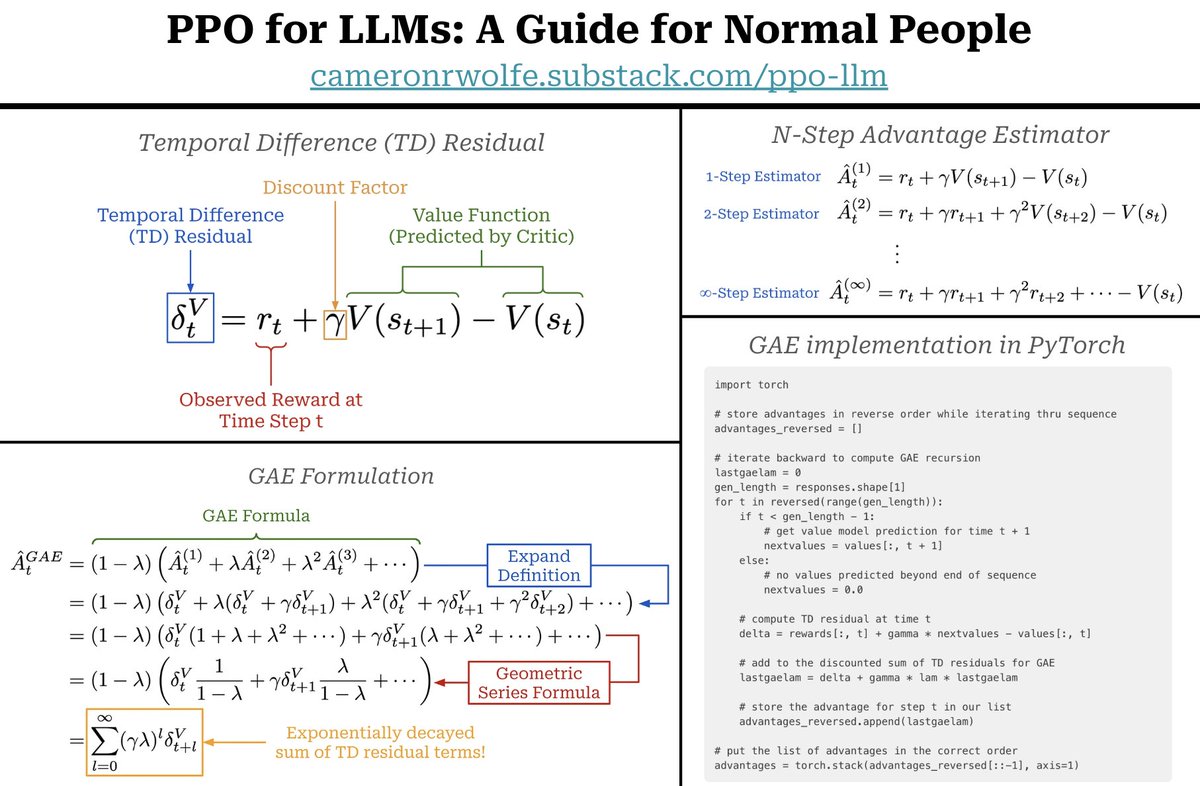
This presents a classic bias-variance trade-off. PPO uses a sophisticated technique called Generalized Advantage Estimation (GAE) to navigate this trade-off. GAE computes the advantage as an exponentially weighted average of k-step advantage estimators, blending the low-variance TD error with the low-bias Monte Carlo return.

The GAE formula is defined using the TD error ${\delta }_t$:

Here, $\lambda \in [0,1]$ is a hyperparameter that controls the trade-off:

• $\lambda =0$: ${\hat{A}}_t={\delta }_t$. This is the high-bias, low-variance TD error.
• $\lambda =1$: ${\hat{A}}_t={\sum }_k{\gamma }^k{\delta }_{t+k}$, which telescopes to the high-variance, low-bias Monte Carlo estimator, $R_t-\hat{V}(s_t)$.

By tuning $\lambda$ (a typical value is ~0.95), we can find a sweet spot that balances bias and variance for efficient and stable learning.

For a concise summary of these concepts, please study the following slide deck extract and image.

Conclusion

In this lesson, we dissected the advantage estimator and its critical function in modern policy gradient methods like PPO.

Here are the key takeaways:

• High Variance: Simple policy gradient estimates that use raw returns are noisy and inefficient, slowing down learning.
• Baselines for Variance Reduction: Subtracting a state-dependent baseline (a control variate) centers the rewards, allowing the agent to distinguish between better-than-average and worse-than-average actions without introducing bias.
• The Critic: The state-value function, $V(s)$, is the ideal baseline. In actor-critic methods, a "critic" network is trained to approximate $V(s)$.
• Generalized Advantage Estimation (GAE): GAE provides a powerful mechanism to estimate the advantage by balancing the bias-variance trade-off between noisy Monte Carlo returns and biased function-approximated values, controlled by the $\lambda$ hyperparameter.

You now have a complete picture of the main components of PPO: the clipped objective for stable updates and the GAE-based advantage estimator for efficient, low-variance updates.

With this foundation, we are perfectly positioned for the next module. We will begin by examining GRPO's main innovation: a critic-free approach. You will learn how GRPO cleverly calculates a relative advantage directly from a batch of model generations, entirely sidestepping the need to train and maintain a separate critic network.