Calculating Model-Weight Memory Requirements

Hello again. In the previous lesson, you traced a request from tokenization through prefill and autoregressive decoding to detokenization. Before any of that request-specific work can happen, the inference engine must keep the model’s learned weights in available device memory.

This lesson gives you the first capacity-planning calculation used in inference engineering: estimating the memory required by model weights from a parameter count and a numerical representation. By the end, you should be able to look at a model described as “8B BF16” or “72B 4-bit” and quickly compute its ideal weight footprint, while recognizing why a real deployment needs additional headroom.

---

Parameters are stored numbers

A model parameter is one learned numeric value in a weight matrix, embedding table, normalization vector, or similar tensor. A model called 8B has roughly $8$ billion such stored values; a 72B model has roughly $72$ billion.

The parameter count tells us how many numbers exist. The numerical format tells us how many bits or bytes are used to store each number. Memory is simply their product.

The essential conversion is:

$$8\text{ bits}=1\text{ byte}$$

If $N$ is the parameter count and $b$ is the number of stored bits per parameter, the ideal raw weight-memory requirement is:

$$M=N\times \frac{b}{8}$$

For model names expressed in billions of parameters, let $P$ denote the number of billions. Using decimal gigabytes, the arithmetic becomes conveniently simple:

$$M_{\mathrm{GB}}\approx P\times \frac{b}{8}$$

This is a weights-only estimate. It answers, “How much memory do the numerical model parameters occupy?” It does not yet account for the cache and temporary runtime state created when requests run.

A useful first reading reinforces this arithmetic and shows the standard rules of thumb.

---

The byte-per-parameter table

For basic inference sizing, memorize this table:

Weight format	Stored bits per parameter	Bytes per parameter	Weight-only rule
FP32	32	4	$4P$ GB
FP16 or BF16	16	2	$2P$ GB
INT8 or 8-bit quantization	8	1	$P$ GB
Nominal 4-bit quantization	4	0.5	$0.5P$ GB

So an $8$B model has an ideal weight footprint of:

• $8\times 4=32$ GB in FP32
• $8\times 2=16$ GB in FP16 or BF16
• $8\times 1=8$ GB in 8-bit form
• $8\times 0.5=4$ GB in nominal 4-bit form

The word ideal matters. These values describe the packed numerical weight values themselves, not a safe hardware requirement. We will distinguish the two carefully later in this lesson.

Why FP16 and BF16 use the same memory but behave differently

Both FP16 and BF16 use $16$ bits, so both require two bytes per stored parameter. Their internal bit allocations differ, however.

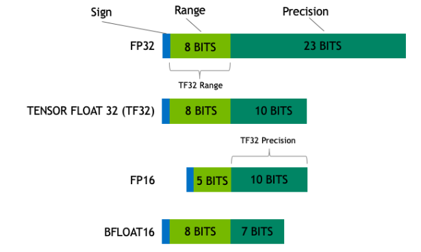
A floating-point number allocates its bits to three roles:

• Sign: whether the number is positive or negative.
• Exponent: the scale or numerical range that can be represented.
• Fraction: the fine-grained precision within that range.

BF16 has an 8-bit exponent, like FP32, but only 7 fraction bits. FP16 has a smaller 5-bit exponent and 10 fraction bits. This distinction can affect numerical behavior, but it does not affect the basic storage calculation: both are $2$ bytes per parameter.

The diagram also includes TF32. Treat TF32 differently from the others for memory planning: it is primarily a GPU computation format used in certain matrix operations, not the usual format in which you choose to store an LLM’s weights. Do not estimate FP32 weight storage as though TF32 made it a 16-bit checkpoint.

---

Deriving the common rules of thumb

It is useful to derive the short rules rather than memorizing disconnected facts.

FP32

FP32 stores each parameter in $32$ bits:

$$\frac{32}{8}=4\text{ bytes per parameter}$$

For a $P$-billion-parameter model:

$$M_{\mathrm{GB}}\approx P\times 4$$

A 72B model in FP32 therefore needs:

$$72\times 4=288\text{ GB}$$

FP16 or BF16

FP16 and BF16 both store each parameter in $16$ bits:

$$\frac{16}{8}=2\text{ bytes per parameter}$$

For a 72B model:

$$72\times 2=144\text{ GB}$$

This is why “roughly 2 GB per billion parameters” is the standard BF16 or FP16 rule.

INT8

With one byte per stored parameter:

$$18\times 1=18\text{ GB}$$

An 18B model in an ideal 8-bit representation occupies about 18 GB of raw weight memory.

Nominal 4-bit quantization

Four bits equal half a byte:

$$\frac{4}{8}=0.5\text{ bytes per parameter}$$

Thus a 200B model at nominal 4-bit weight precision has this theoretical raw footprint:

$$200\times 0.5=100\text{ GB}$$

The calculation is linear: doubling parameters doubles required weight storage; halving stored bits per parameter halves it.

---

Read the chart as a linear scaling law

The following chart visualizes precisely that relationship across several parameter counts and bit widths.

Pick one bar and verify it mentally. The 72B model at 16-bit precision is shown at 144 GB:

$$72\times 2=144\text{ GB}$$

The 500B model at 4-bit precision is shown at 250 GB:

$$500\times 0.5=250\text{ GB}$$

The chart makes two operational facts immediately visible:

1. Parameter count dominates. A modest change in numerical format cannot make a very large model small. Even 4-bit storage for a 500B model is about 250 GB of raw weights.
2. Precision has a large linear effect. Moving from FP16 to 4-bit reduces ideal raw weight storage by a factor of four.

The 64-bit bars are mathematically correct but are mostly illustrative. FP64 is generally not a practical weight format for LLM inference, since its eight bytes per parameter create an enormous footprint without offering an inference-serving benefit proportionate to that cost.

---

Decimal GB, binary GiB, and why “fits” is not enough

Hardware vendors usually advertise memory in decimal gigabytes:

$$1\text{ GB}=10^9\text{ bytes}$$

Many operating-system tools instead display gibibytes:

$$1\text{ GiB}=2^{30}\text{ bytes}$$

For example, exactly 16 billion bytes is:

$$\frac{16\times 10^9}{2^{30}}\approx 14.9\text{ GiB}$$

This does not mean an 8B FP16 model comfortably fits on a “16 GB” GPU. It means the two displays use different units for nearly the same physical capacity. The raw FP16 weights still require about 16 decimal GB, leaving essentially no room for anything else.

For fast engineering estimates:

• use the model’s quoted billions of parameters with decimal GB;
• compare with the device’s advertised decimal GB;
• leave substantial capacity beyond the raw weight number.

If you need high-confidence deployment sizing, inspect the actual model artifact and measure the running process. The simple formula is your first filter, not the final approval.

---

Weight footprint versus real runtime memory

A model that has a 16 GB weight footprint does not require only 16 GB of device memory in practice. The inference process also uses memory for items such as:

• the KV cache, which grows with active sequence length and concurrent requests;
• temporary activations and workspace used during computation;
• runtime and framework allocations;
• GPU driver and kernel-related allocations;
• quantization metadata, such as scales and zero-points;
• occasionally, weights retained at a different precision by a particular engine.

For this reason, use the formula in this lesson in two stages:

1. Feasibility screen: Do the weights alone fit in the target memory?
2. Deployment plan: Is there enough remaining space for runtime overhead and the intended workload?

If the weights alone exceed capacity, the model cannot run entirely on that device in that format. If the weights just equal capacity, the deployment is also not viable without changing the format, reducing the model, splitting it across devices, or using a system that supports partial offload.

The next lesson will quantify the most important request-dependent part of that remaining budget: the KV cache.

---

What “4-bit” really means

The formula for 4-bit weights is intentionally a first-order estimate, not a promise that every 4-bit model file will be exactly $0.5P$ GB.

A normal floating-point tensor stores each parameter directly as a standard numeric value. Quantized formats instead store a compact code for each weight plus enough extra information to reconstruct an approximation during computation. That extra information can include per-group scales, zero-points, lookup tables, or format-specific metadata.

Therefore, for a quantized model:

$$\text{actual weight storage}\gtrsim \text{nominal bits per parameter estimate}$$

A 4-bit artifact can be somewhat larger than the ideal $0.5$ bytes per parameter. Different quantization formats can also make different trade-offs among:

• actual memory use,
• output quality,
• compatibility with an inference engine,
• and speed on a particular CPU, GPU, or Apple Silicon system.

For the present calculation, treat “4-bit” as approximately 0.5 GB per billion parameters, then verify the actual artifact size and runtime usage before committing to hardware.

The same caution applies to a model’s advertised parameter count. For ordinary dense models, “8B” is usually a useful approximation. For architectures with experts, capacity planning must use the total parameters that are actually loaded into memory, not only the smaller number of parameters active for one token.

---

A short calculation workflow

When evaluating a candidate model, apply this workflow:

1. Find the model’s total loaded parameter count. Use the model documentation, not the context-window size or the number of layers.
2. Identify the weight representation. Examples include BF16, FP16, 8-bit, or a named 4-bit quantization format.
3. Convert format to bytes per parameter. FP16 and BF16 mean 2; 8-bit means 1; nominal 4-bit means 0.5.
4. Multiply parameter billions by bytes per parameter. This produces the raw decimal-GB weight estimate.
5. Treat the result as a lower bound. Check actual artifact size, runtime documentation, and the memory required for active requests.

For instance, suppose your target has 24 GB of usable accelerator memory:

Candidate	Ideal raw weights	Initial conclusion
8B BF16	16 GB	Weight fit is possible, but remaining memory may be tight
18B 8-bit	18 GB	Possible in principle, with limited runtime headroom
18B FP16	36 GB	Does not fit on one 24 GB device
72B 4-bit	36 GB	Does not fit on one 24 GB device despite quantization
8B 4-bit	4 GB	Leaves considerably more room for runtime state

Notice what this table does not claim: it does not say that a format that fits will be fastest, best quality, or suitable for a particular number of simultaneous users. It answers only the correct first question: Can the raw weights plausibly reside in the available memory?

The following short video applies the same calculation to a much larger model and illustrates why format choice can change the required hardware tier.

---

Key takeaways

• Raw model-weight memory is determined by parameter count multiplied by bytes per parameter.
• For a $P$-billion-parameter model, use $4P$ GB for FP32, $2P$ GB for FP16 or BF16, $P$ GB for 8-bit, and approximately $0.5P$ GB for nominal 4-bit weights.
• FP16 and BF16 occupy the same memory, even though their exponent and fraction-bit allocations differ.
• A raw weight calculation is a lower bound, not a full serving-memory estimate. Runtime overhead and request-dependent state also consume memory.
• Quantized models reduce weight memory substantially, but their actual artifact and runtime footprints include metadata and vary by format and engine.
• A model that merely matches device capacity does not safely fit for inference; it needs room for real runtime operation.

Next, you will extend this memory budget beyond persistent weights by calculating KV-cache memory from architecture dimensions, context length, batch size, and precision.