Understanding Mamba and State Space Models as Transformer Alternatives

Hello! Welcome to the first lesson of our new module, Emerging Architectures and Research Frontiers.

In our previous modules, we've built a strong foundation, covering everything from core machine learning concepts to the intricacies of the Transformer architecture and the distributed training strategies needed to scale them. We concluded by exploring how to train massive models across many GPUs. Now, we shift our focus from how to train existing architectures to what comes next.

For years, the Transformer has been the undisputed king of sequence modeling, but its quadratic complexity in self-attention presents a significant bottleneck for handling very long sequences. This lesson addresses the learning outcome: Analyze the architecture of State Space Models like Mamba as an alternative to Transformers. We will investigate a new class of models that promises Transformer-level performance with linear-time complexity, re-introducing ideas from classical control theory in a modern deep learning context.

Our journey will cover:

1. The "Why": Understanding the limitations of Transformers that motivate the search for alternatives.
2. State Space Models (SSMs): Introducing the core concepts, rooted in continuous-time systems.
3. From Continuous to Discrete: How SSMs are adapted for digital computation and sequence data using recurrent and convolutional representations.
4. Handling Long Dependencies: The role of the HiPPO framework and the S4 model.
5. Mamba's Innovations: The key breakthroughs of selectivity and hardware-aware parallelism that make SSMs competitive.
6. The Mamba Architecture: A detailed look at the components of a Mamba block.

Let's dive into this exciting new frontier of model architecture.

---

1. Beyond the Transformer: The Quest for Linear Time

As we've discussed, the power of the Transformer lies in its self-attention mechanism, which allows every token to directly attend to every other token in the sequence. This provides a rich, uncompressed view of the context. However, this comes at a cost.

• Quadratic Complexity: The attention matrix for a sequence of length $L$ has dimensions $L\times L$. This means both the computational and memory requirements scale quadratically, i.e., $O(L^2)$. Doubling the sequence length quadruples the cost of the attention layer.
• Inference Bottleneck: During autoregressive generation, the Key-Value (KV) cache grows with each new token, making inference on very long sequences memory-intensive and slow.

This scaling issue has fueled a search for new architectures that can match the Transformer's power while scaling linearly, $O(L)$, with sequence length. One of the most promising candidates is the State Space Model.

---

2. What is a State Space Model (SSM)?

State Space Models are not new; they originate from control theory and have been used for decades in fields like electrical and mechanical engineering to model dynamic systems. The core idea is to represent a system using a latent state variable that summarizes the entire history up to the present moment.

The evolution of this state and the resulting output are described by a pair of linear ordinary differential equations (ODEs):

1. The State Equation: Describes how the latent state $x(t)$ changes over time.
   $x^{\prime }(t)=Ax(t)+Bu(t)$
2. The Output Equation: Describes how the latent state $x(t)$ is translated into an output $y(t)$.
   $y(t)=Cx(t)+Du(t)$

Here:

• $u(t)$ is the continuous input signal.
• $x(t)$ is the latent state vector (of size $N$).
• $y(t)$ is the output signal.
• $A,B,C,D$ are matrices that define the system's dynamics. They are the parameters of the model.

Your physics background might appreciate a concrete example. The motion of a simple spring-mass-damper system can be perfectly described by these equations, where $u(t)$ is an applied force, and the state $x(t)$ might contain the mass's position and velocity.

---

3. Adapting SSMs for Deep Learning

The continuous-time formulation is elegant, but deep learning operates on discrete data like tokens. To bridge this gap, SSMs need to be adapted through a process called discretization.

Discretization and the Two Computational Views

Discretization converts the continuous ODEs into discrete recurrence relations that operate on sequences. A common method is the Zero-Order Hold (ZOH), which assumes the input signal is constant between discrete time steps. This process transforms the continuous matrices $A$ and $B$ into their discrete counterparts, $\bar{A}$ and $\bar{B}$, using a new hyperparameter, the step size $\Delta$.

This gives us the following sequence-to-sequence equations, where $k$ is the timestep index:

$x_k=\bar{A}{x}_{k-1}+\bar{B}{u}_k$
$y_k=\bar{C}{x}_k$

This discrete formulation can be computed in two different but equivalent ways, giving rise to a powerful duality.

To summarize the two computational views:

1. Recurrent Mode: The discrete state equation is identical to the formulation of a simple Recurrent Neural Network (RNN).

   • Pros: Extremely fast and memory-efficient during inference. To generate the next token, you only need the previous state $x_{k-1}$ and the current input $u_k$. The state size is fixed, so it scales linearly $O(L)$ with sequence length and has a theoretical infinite context.
   • Cons: Training is sequential and slow, as each step depends on the previous one, making it difficult to parallelize on GPUs.

2. Convolutional Mode: By unrolling the recurrence, the entire output sequence $y$ can be computed in one go as a convolution of the input sequence $u$ with a specially constructed kernel $\bar{K}$.

   • $\bar{K}=(\bar{C}\bar{B},\bar{C}\bar{A}\bar{B},\bar{C}{\bar{A}}^2\bar{B},\dots )$
   • $y=\bar{K}\ast u$
   • Pros: Convolutions are highly parallelizable on GPUs, making training very fast.
   • Cons: The convolution kernel $\bar{K}$ can be very large (equal to the sequence length), and inference is inefficient as it requires re-computing over the whole context.

This duality allows for the best of both worlds: train in parallel using the convolution mode, then perform efficient inference using the recurrent mode.

---

4. S4: Structuring the State for Long-Range Memory

A vanilla SSM, even with the convolution/recurrence trick, struggles to model long-range dependencies. The problem lies in the state matrix $A$. If not structured properly, it can cause the state $x$ to either explode or vanish over long sequences, effectively "forgetting" early information.

The solution comes from a framework called HiPPO (High-order Polynomial Projection Operators). The deep mathematical details are complex, but the intuition is that HiPPO provides a principled way to initialize the $A$ matrix so that the state $x(t)$ optimally compresses the history of the input signal $u(t)$ by tracking the coefficients of a polynomial basis (e.g., Legendre polynomials).

This structured initialization of matrix $A$ ensures that the SSM can effectively remember information over very long distances. Combining this HiPPO theory with the SSM framework gives rise to the Structured State Space for Sequences (S4) model.

S4 models were the first to demonstrate that properly structured SSMs could compete with and even outperform Transformers on benchmarks involving long dependencies.

---

5. Mamba's Breakthrough: The Selective SSM (S6)

While S4 was a huge step, it still had a critical limitation: it is Linear Time-Invariant (LTI). The matrices $\bar{A}$, $\bar{B}$, and $\bar{C}$ are fixed for all time steps and are independent of the input. This means the model cannot reason about the content of the input; it processes every token using the same dynamics, making it struggle with tasks that require context-aware decisions (like ignoring filler words or recalling a specific fact mentioned earlier).

Mamba solves this by introducing selectivity, turning the SSM into a time-variant system.

Mamba's two key contributions form the Selective SSM (S6) architecture:

1. Selectivity Mechanism: Mamba makes the matrices $\bar{B}$, $\bar{C}$, and the step size $\Delta$ input-dependent. For each input token $u_k$, a small network projects it to generate specific ${\bar{B}}_k$, ${\bar{C}}_k$, and ${\Delta }_k$ for that time step. This allows the model to dynamically decide how much of the current input to ingest into the state and how to project that state to the output, effectively "selecting" what information to remember or ignore based on content.

2. Hardware-Aware Parallel Algorithm: This input-dependency breaks the convolution trick, as the kernel is no longer fixed. A naive recurrent implementation would be too slow for training. Mamba's authors solved this with a two-pronged approach:

   • Parallel Scan: They use a parallel scan algorithm, an alternative to convolution, which restructures the sequential recurrence $x_k=f(x_{k-1},u_k)$ to be computed in logarithmic time on parallel hardware. Your CS background will appreciate this as an application of parallel prefix sum algorithms to a more complex associative operator.
   • Kernel Fusion: To overcome the memory I/O bottleneck of moving data between the large but slow GPU HBM and the small but fast SRAM, they fuse the entire SSM computation (discretization, scan, and output projection) into a single GPU kernel. This minimizes data movement and dramatically speeds up execution, a concept we touched on when discussing FlashAttention.

This S6 model is powerful, content-aware, and maintains linear-time scaling, making it a true contender to the Transformer.

Test your understanding!

During autoregressive inference, how does the computational and memory complexity of a Transformer compare to that of a Mamba model as the generated sequence gets longer? Why?

Show answer

• Transformer: Both computational and memory complexity scale quadratically, $O(L^2)$, with sequence length $L$. This is because the attention mechanism requires re-evaluating the query against a growing Key-Value (KV) cache that stores information for all previous tokens.

• Mamba: Both computational and memory complexity scale linearly, $O(L)$. This is because Mamba operates in its recurrent mode during inference. To generate the next token, it only needs the fixed-size hidden state from the previous step and the current input. It does not need to store and re-process the entire history, as all relevant information is compressed into the state vector.

---

6. The Mamba Block Architecture

The S6 layer is the core of Mamba, but like the self-attention layer in a Transformer, it's embedded within a larger block structure.

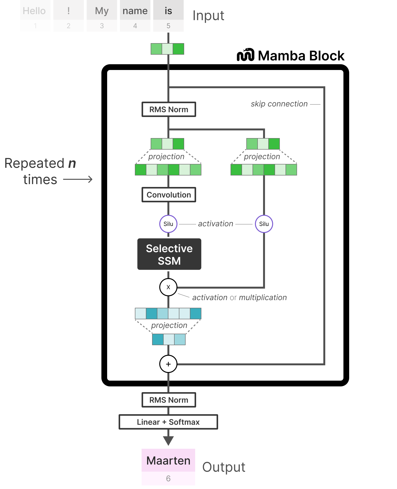
Let's trace the flow of data through a Mamba block:

1. Input & Normalization: The input sequence first passes through a normalization layer (typically RMSNorm).
2. Expansion & Gating: A linear layer projects the input into a higher-dimensional space and splits it into two paths. One path will go through the main SSM logic, while the other will act as a "gate."
3. Convolution: The main path first passes through a 1D convolution. This allows the model to mix information from nearby tokens before the SSM processes them sequentially.
4. Activation: A SiLU (Sigmoid-weighted Linear Unit) activation is applied.
5. Selective SSM (S6): The data then flows through the S6 layer, which performs the selective state update and output generation as described above.
6. Gating: The output of the S6 layer is modulated by the second path (the "gate") using element-wise multiplication. This is a common pattern in modern architectures (like in GLU activations) that gives the network more control over the information flow.
7. Output Projection: Finally, a linear layer projects the result back down to the model's residual dimension.

Like Transformer blocks, these Mamba blocks are stacked, with residual connections adding the block's input to its output, to form a deep model.

---

Conclusion

In this lesson, we've explored the exciting architecture of State Space Models and Mamba, a powerful alternative to the Transformer.

Key Takeaways:

• SSMs are inspired by classical control theory and use a latent state to model sequences.
• They have a dual representation: a recurrent mode for efficient inference and a convolutional mode for parallelizable training.
• The S4 model introduced the HiPPO framework to structure the state matrix $A$, enabling it to handle long-range dependencies effectively.
• Mamba introduces selectivity by making its parameters input-dependent, allowing for content-aware reasoning.
• Mamba remains fast thanks to a hardware-aware parallel scan algorithm, achieving $O(L)$ complexity in both training and inference while matching Transformer performance.

Mamba represents a significant architectural innovation, demonstrating that there are powerful sequence modeling paradigms beyond attention. It marks a potential resurgence of RNN-like ideas, re-imagined for the era of large-scale deep learning and modern hardware.

Preview of the Next Lesson:

Now that we've seen how a cutting-edge architecture is designed, our next step is to look inside the "black box." How can we understand the reasoning behind a model's predictions? In the next lesson, we will begin exploring model interpretability by implementing gradient-based attribution methods like saliency maps and Integrated Gradients.