Quantum Error Mitigation vs. Quantum Error Correction

Hello! Welcome to the next lesson in your deep dive into recent advances in quantum computing.

In our last lesson, we analyzed Gottesman-Kitaev-Preskill (GKP) codes, a sophisticated example of active Quantum Error Correction (QEC). We saw how their unique grid structure in phase space allows for the detection and correction of small displacement errors in real time, provided one has access to high-quality ancillary states. This approach is part of the long-term vision for building fault-tolerant quantum computers.

Today, we pivot to a different, more pragmatic strategy designed for the quantum computers we have today. This lesson will introduce you to the principles of Quantum Error Mitigation (QEM), a set of techniques that don't try to prevent or fix errors on the fly, but rather to estimate and computationally remove their effects from the final result. This directly addresses the learning outcome: Describe the principles of quantum error mitigation as a strategy for near-term quantum devices, contrasting it with quantum error correction.

By the end of this lesson, you'll understand the fundamental philosophical and practical differences between QEC and QEM, and you will be familiar with the core ideas behind two leading mitigation techniques.

1. A Tale of Two Strategies: Error Correction vs. Error Mitigation

The central challenge in quantum computing is decoherence and noise. Quantum Error Correction (QEC) and Quantum Error Mitigation (QEM) represent two distinct philosophies for tackling this challenge.

As the paper highlights, the distinction boils down to goals and resources:

• Quantum Error Correction (QEC):

  • Goal: To achieve fault tolerance. The aim is to encode a "logical" qubit into many physical qubits, actively detect and correct errors, and thus protect the logical information indefinitely, provided the physical error rate is below a certain threshold.
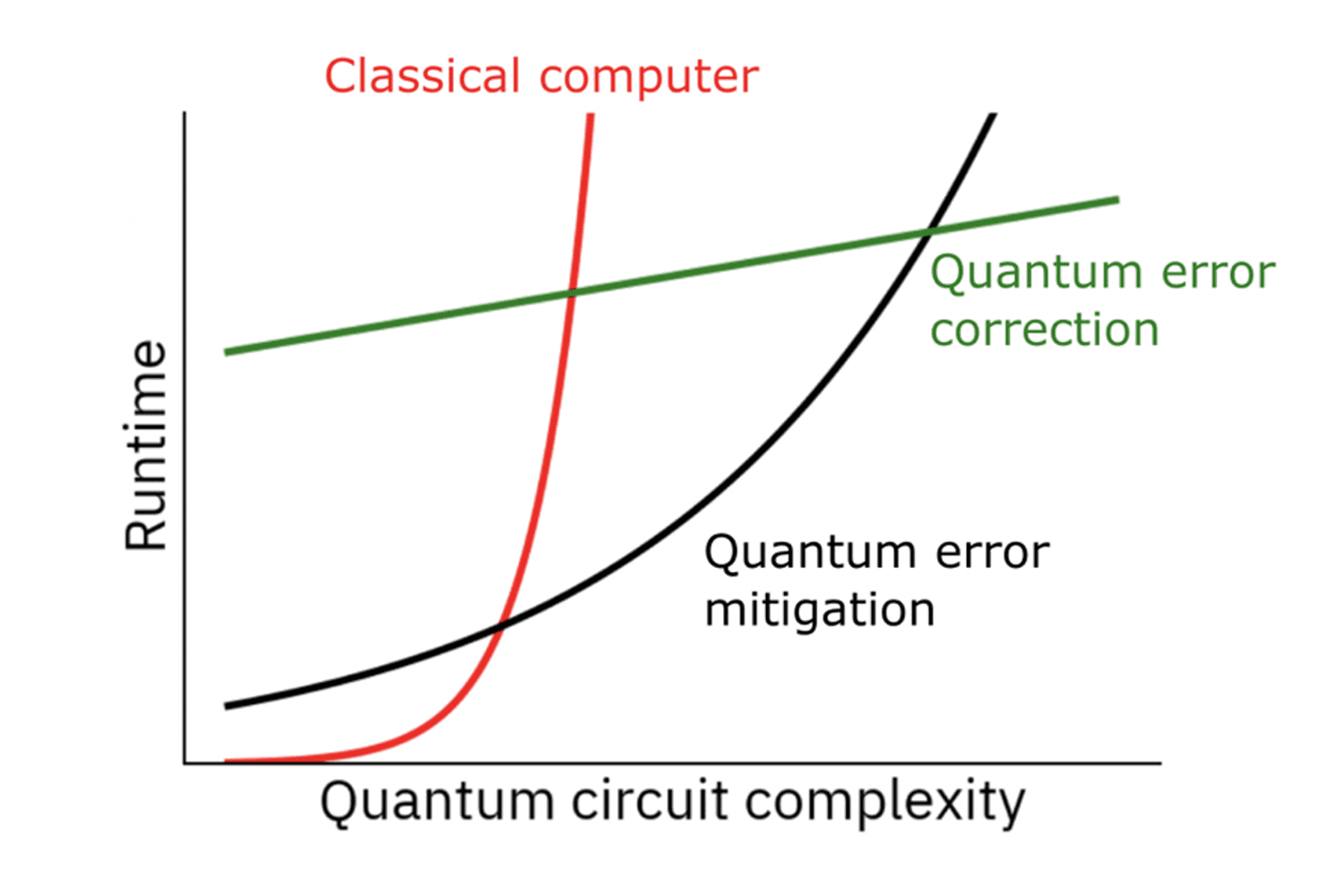
  • Resources: Extremely high overhead in the number of physical qubits. As mentioned in the paper, estimates suggest $\sim 1000$ physical qubits might be needed per logical qubit for useful fault-tolerant computation. This makes it a long-term goal.

• Quantum Error Mitigation (QEM):

  • Goal: To improve the accuracy of an expectation value for a specific, short-depth quantum circuit. It acknowledges that errors will happen and seeks to estimate their aggregate effect and subtract it via classical post-processing. It does not create a stable logical qubit.
  • Resources: Low overhead in qubit count (it uses the same qubits as the unmitigated circuit), but it incurs a "sampling overhead" by requiring more measurements and/or more complex classical processing. This makes it suitable for Noisy Intermediate-Scale Quantum (NISQ) devices.

This fundamental trade-off is beautifully summarized in the following conceptual graph.

Now, let's delve into the principles of the two most prominent QEM techniques.

2. Principle 1: Zero-Noise Extrapolation (ZNE)

The core idea of ZNE is remarkably intuitive: if you can't get rid of the noise, what if you could controllably increase it? By observing how the output changes as you dial up the noise, you can extrapolate backwards to a hypothetical zero-noise result.

To put this on a more formal footing, let's look at the implementation details.

The ZNE protocol consists of three main steps:

1. Noise Scaling: We execute the circuit not just once, but multiple times, each time with a different, artificially increased level of noise. A common way to do this is called unitary folding. To double the noise from a circuit $U$, you can run the sequence $U{U}^{†}U$. Since $U^{†}U=I$ ideally, this sequence is logically equivalent to $U$, but it executes twice the number of gates, thereby approximately doubling the accumulated noise. For a noise scale factor $\lambda$, we can append $(\lambda -1)/2$ pairs of $U^{†}U$.

2. Measurement: For each noise scale factor ${\lambda }_i$, we measure the expectation value of our observable, $⟨O{⟩}_{{\lambda }_i}$. This gives us a set of data points $({\lambda }_i,⟨O{⟩}_{{\lambda }_i})$. The native hardware noise corresponds to ${\lambda }_1=1$.

3. Extrapolation: We fit a model to these data points (e.g., a linear or polynomial function) and use it to extrapolate to the y-intercept where the noise is zero ($\lambda =0$). This extrapolated value is our mitigated estimate of the expectation value. For an extrapolation using $k$ noise levels, the final result is a linear combination:

   $$⟨O{⟩}_{\text{ZNE}}=\sum _{i=1}^k{\eta }_i⟨O{⟩}_{{\lambda }_i}$$

   where the coefficients ${\eta }_i$ depend on the chosen extrapolation model (e.g., Richardson extrapolation, as seen in Eq. (8) of the paper LINK).

Key feature of ZNE: It is model-free. You don't need to know the specifics of the noise affecting your device; you only need a way to amplify it. This makes it very general, but as noted in the Mitiq documentation, the result can be sensitive to the choice of extrapolation model and noise scaling method.

3. Principle 2: Probabilistic Error Cancellation (PEC)

PEC is a more powerful, but also more demanding, technique. Instead of just observing the effects of noise, it attempts to actively cancel it on average.

The analogy to noise-canceling headphones is very apt: those headphones listen to the ambient noise and generate an "anti-noise" sound wave to cancel it. PEC works by first learning a precise model of the noise and then probabilistically inserting operations into the circuit that, on average, perform the inverse of the noise operation.

Let's summarize the profound concepts from that video:

• The Goal and the Problem: An ideal gate is $G_{\text{ideal}}$. On a real device, you implement a noisy operation $\mathcal{E}$ which can be thought of as the ideal gate followed by a noise channel, $\mathcal{E}=\Lambda \circ G_{\text{ideal}}$. To undo the noise, we'd want to apply the inverse map, ${\Lambda }^{-1}$. However, noise channels are trace-preserving, completely-positive (CPTP) maps that shrink the Bloch sphere (representing loss of information/purity). Their inverse would have to expand the Bloch sphere, which is not a physical quantum operation.

• The Quasi-probability Solution: The key insight of PEC is that we can express the ideal gate $G_{\text{ideal}}$ as a linear combination of the noisy, implementable operations $\{{\mathcal{E}}_{\alpha }\}$ that our hardware can actually perform:

  $$G_{\text{ideal}}=\sum _{\alpha }{\eta }_{\alpha }{\mathcal{E}}_{\alpha }$$

  Some of the coefficients ${\eta }_{\alpha }$ can be negative. These are not true probabilities, but quasi-probabilities.

• Implementation: To run the ideal circuit, for each gate $G_{\text{ideal}}$, we randomly choose to execute one of the physical operations ${\mathcal{E}}_{\alpha }$ with probability $p_{\alpha }=|{\eta }_{\alpha }|/\gamma$, where $\gamma ={\sum }_{\alpha }|{\eta }_{\alpha }|$ is a normalization factor. We then run this randomly generated circuit and measure our observable. The crucial step is that we multiply the measurement outcome by $\text{sign}({\eta }_{\alpha })$ in classical post-processing. When averaged over many such random circuits, the contributions from the negative ${\eta }_{\alpha }$ terms correctly subtract out, and the expectation value converges to the ideal, noise-free value.

• The Cost: This doesn't come for free. The factor $\gamma$ is the sampling overhead. The number of total shots required to achieve a certain precision scales as ${\gamma }^2$. For a circuit with $L$ gates, the total overhead ${\gamma }_{\text{tot}}={\prod }_{i=1}^L{\gamma }_i$ grows exponentially with the circuit depth. This is the primary limitation of PEC.

Conclusion

This lesson has drawn a clear distinction between the long-term goal of quantum error correction and the near-term necessity of quantum error mitigation.

Key Takeaways:

• QEC vs. QEM: QEC aims for fault tolerance by actively correcting errors with high qubit overhead. QEM aims for improved accuracy on NISQ devices by computationally subtracting noise effects with high sampling overhead.
• Zero-Noise Extrapolation (ZNE): A model-free technique that works by amplifying noise in a controlled way and extrapolating the results back to the zero-noise limit. Its strength is its generality.
• Probabilistic Error Cancellation (PEC): A model-based technique that learns a precise noise model to implement the inverse noise channel on average via quasi-probability sampling. It can provide an unbiased estimate but suffers from an exponential sampling cost with circuit depth.
• The NISQ Strategy: QEM is a crucial strategy for extracting value from today's noisy quantum processors. It represents a trade-off: using increased classical computation and measurement shots to compensate for the imperfections of the quantum hardware.

Preview of the next lesson:
Having established the theoretical principles, our next two lessons will make these concepts concrete. In the upcoming lesson, we will focus on implementing zero-noise extrapolation (ZNE) for a simple quantum circuit. You will get hands-on experience with noise scaling and see how the extrapolation process improves the final result on a noisy simulator.