Concentrated Liquidity: Capital Efficiency and LP Risk

Welcome back. Previously, you separated an LP’s result into trading fees, token incentives, impermanent loss, and operational costs. That decomposition remains essential here: concentrated liquidity does not remove impermanent loss or make fee income guaranteed. It changes where your capital is available for trading, making the return profile more efficient when your range is active and more conditional when it is not.

This lesson explains that trade-off using Uniswap v3-style concentrated liquidity. You will be able to distinguish capital efficiency from “high yield,” track how a position’s inventory changes across its chosen price range, and identify the new risks created by choosing—and maintaining—a range.

---

From liquidity everywhere to liquidity where trading occurs

A full-range constant-product pool makes liquidity available across every theoretically possible price. That is useful: whatever price the asset reaches, the pool still has liquidity and its LPs remain active. But it is also capital-intensive.

Consider a DAI/USDC pool. Most trading should occur close to $1$ USDC per DAI. Capital allocated to support prices far away from parity is unlikely to be used under normal conditions. In a full-range design, however, an LP commits funds to the entire price curve anyway.

Concentrated liquidity lets an LP select a lower and upper price bound. The LP’s capital is then used only inside that interval.

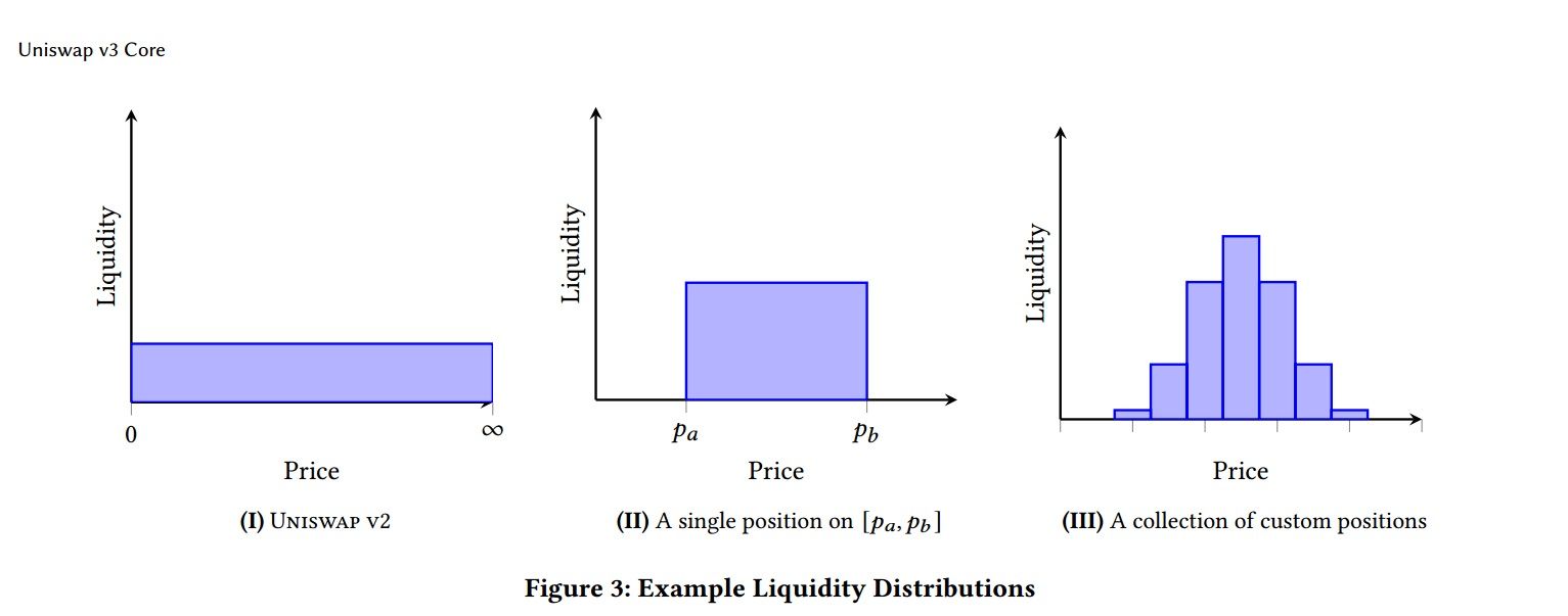
For example, rather than supply DAI/USDC liquidity from effectively zero to infinity, an LP may choose the range:

$$0.98\le P_{\text{DAI in USDC}}\le 1.02$$

Within that range, the position provides much greater trading depth per dollar committed than a comparable full-range position. For a stablecoin pair that mostly trades near parity, this is an economically sensible allocation: it directs capital toward the prices at which traders are likely to transact.

What “capital efficiency” actually means

Capital efficiency is not the same as profit, annual percentage rate, or safety. In this context, it means:

How much usable liquidity depth can the protocol offer near the current trading price for each dollar an LP commits?

A narrower active range generally means more depth at the current price for the same deposit. Equivalently, an LP can often commit less capital to achieve similar near-price depth.

This has two distinct implications:

Question	Full-range liquidity	Concentrated liquidity
Where is capital available?	Across all possible prices	Only within chosen intervals
Depth near current price per deposited dollar	Lower	Higher while in range
Capital required for similar near-price depth	Higher	Potentially lower
Does the position earn fees continuously?	Usually, as long as the pool trades	Only while its range is active
Management required	Relatively passive	Range selection and possible repositioning

The word potentially matters. A narrowly concentrated LP does not automatically earn more fees in dollar terms. Its actual fee income depends on:

• whether price stays in the range;
• how much trading volume occurs while it is in range;
• its share of active liquidity relative to competing LPs;
• the pool’s fee tier;
• gas and rebalancing costs;
• the extent to which arbitrage-driven trading compensates for the inventory risk.

So the accurate claim is not “tight ranges create high returns.” It is:

Tight ranges can produce more fee-generating liquidity per unit of committed capital while the market price remains in that range.

---

A position is a range-dependent inventory strategy

In a conventional full-range pool, an LP holds both assets at practically every ordinary price. In a concentrated position, the asset mix is tied much more explicitly to the chosen lower and upper bounds.

Suppose an LP supplies DAI and USDC in the range $0.98$ to $1.02$ USDC per DAI.

There are three price regions.

Market price of DAI	Position status	Typical asset composition	Fees
Below $0.98$ USDC	Out of range	100% DAI	No new fees
Between $0.98$ and $1.02$ USDC	Active	A mixture of DAI and USDC	Earns fees
Above $1.02$ USDC	Out of range	100% USDC	No new fees

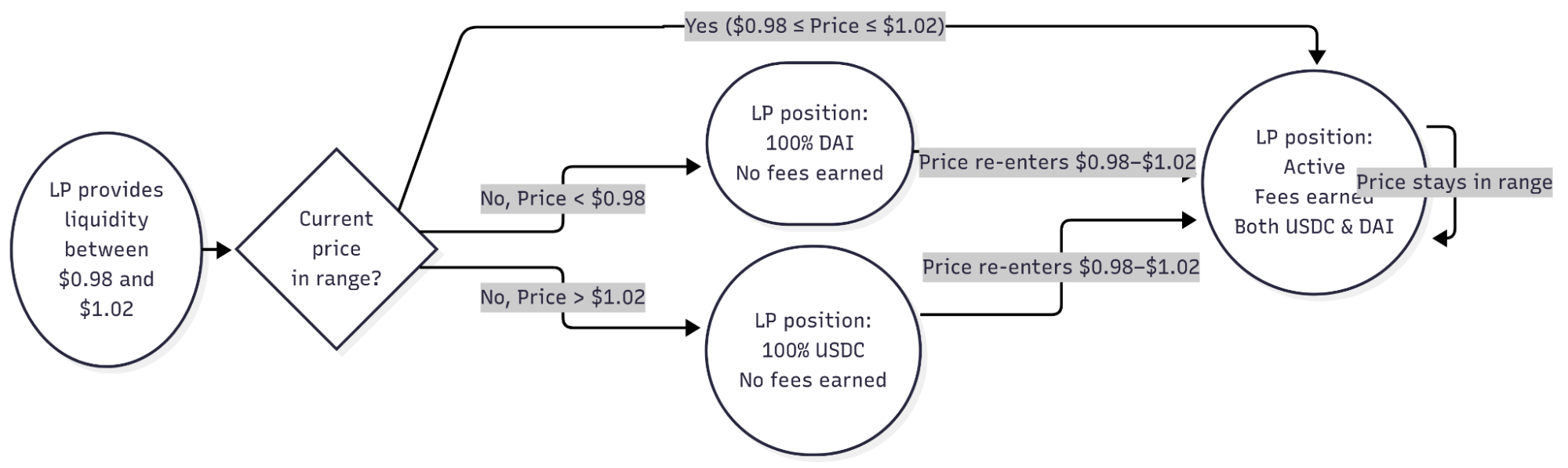
The direction of conversion follows the AMM’s trading activity:

• If DAI falls relative to USDC, traders exchange DAI into the pool and withdraw USDC. The LP increasingly holds DAI. Once price passes below the lower bound, the position is entirely DAI.
• If DAI rises relative to USDC, traders exchange USDC into the pool and withdraw DAI. The LP increasingly holds USDC. Once price passes above the upper bound, the position is entirely USDC.

This is the concentrated version of the rebalancing behavior you saw in the prior lesson. The LP is still systematically selling the asset rising relative to its pair and accumulating the asset falling relative to its pair. Concentration makes the process bounded: after one edge of the range is crossed, the position has completed its conversion into a single asset.

A useful way to interpret this is that an LP has not merely chosen two tokens. They have chosen:

1. a pair of tokens;
2. a price interval;
3. a degree of willingness to rebalance between those tokens;
4. a plan, explicit or implicit, for what happens if price leaves that interval.

---

Why narrow ranges raise the stakes

Narrowing a range is the central trade-off. It increases capital efficiency, but it also reduces the room for normal price movement before the position becomes inactive.

Imagine two DAI/USDC LPs with the same initial deposit value:

• Wide-range LP: $0.90$ to $1.10$ USDC per DAI
• Narrow-range LP: $0.99$ to $1.01$ USDC per DAI

The narrow-range LP supplies substantially more depth around parity per dollar deposited. But a modest depeg that is irrelevant to the wide-range LP can put the narrow-range LP fully out of range.

This is the central risk-return relationship:

Narrower range	Wider range
More liquidity depth near current price	Less liquidity depth near current price
Larger potential fee share per dollar while active	Lower potential fee share per dollar while active
Less tolerance for price movement	More tolerance for price movement
Faster conversion toward one asset	More gradual inventory change
More likely to require intervention	Less frequent need to reposition

Concentrated liquidity and impermanent loss

The previous lesson defined impermanent loss as the LP position’s underperformance versus holding the original token quantities. That comparison still applies, but a concentrated position has a more range-dependent payoff.

While the price moves within a narrow interval, the position’s inventory can change rapidly relative to its committed capital. When the price reaches a bound, the LP holds one token only. The result is often described as an amplification of impermanent-loss risk, but the more precise statement is:

Concentration makes the LP’s relative performance more sensitive to price movement across the chosen range and can leave the LP fully exposed to one asset after a boundary is crossed.

For the DAI/USDC position:

• Below $0.98$, the LP is entirely exposed to DAI. If DAI continues falling, the LP bears that DAI exposure with no new fee income from this position.
• Above $1.02$, the LP is entirely exposed to USDC. If DAI continues rising, the LP no longer participates in that upside because it has already sold its DAI into USDC through AMM rebalancing.

This does not mean every out-of-range position has an immediate dollar loss. If the position becomes all USDC after DAI rises, its USDC value may be stable or even higher than at deposit. But compared with holding the initial DAI amount, it can underperform further if DAI keeps appreciating. The benchmark remains the original asset quantities.

---

The risks introduced by range selection

Concentrated liquidity turns an LP position from a relatively passive exposure into something closer to a standing, rule-based market-making strategy. That introduces several risks beyond the familiar full-range impermanent-loss effect.

1. Out-of-range risk

Once price leaves the chosen interval, the position is inactive:

• it no longer contributes liquidity at the current price;
• it earns no additional swap fees;
• it holds only one asset;
• it may stay inactive for a long time.

An LP can leave the position unchanged and wait for price to re-enter. That avoids immediate transaction costs but leaves capital idle from a fee-generation perspective. Alternatively, the LP can withdraw and create a new range around the current price. That restores activity but incurs costs and locks in the position’s current composition.

2. Directional inventory risk

A range position is not neutral simply because it began with two tokens. The AMM’s rebalancing creates a directional outcome:

• a decline through the lower bound leaves the LP holding the declining asset;
• a rise through the upper bound leaves the LP holding the asset that did not rise.

This is often undesirable if the LP’s real objective was simply to retain a balanced portfolio. It may be desirable, however, if the LP deliberately wants to sell an asset at higher prices or accumulate it at lower prices. The same mechanics can function like a gradual range order, but that is a strategy choice—not a free improvement in returns.

3. Fee uncertainty and adverse selection

Fees are compensation for providing immediacy to traders. Some trading is uninformed and may be relatively favorable for LPs. But rapid price changes often attract arbitrageurs who trade against the pool as its quoted price catches up to the broader market.

That arbitrage is necessary for the AMM price to track the market, yet it is also the mechanism through which the LP’s inventory shifts. A pool can show substantial volume and fees while LPs still have poor net outcomes if the price moves persistently in one direction.

The relevant question is therefore not:

“Is the fee APR high?”

It is:

“Were the fees earned during the same period sufficient compensation for the position’s inventory change, divergence from holding, and operating costs?”

4. Active-management and transaction-cost risk

A tightly concentrated position may need frequent repositioning to remain active. That creates several practical costs:

• gas for withdrawing and minting or modifying positions;
• possible swap costs if the LP wants a different token mix for the new range;
• time and monitoring burden;
• execution risk during volatile moves;
• dependence on an automated manager, if one is used.

Automation changes who performs the range management; it does not remove the economic trade-off. An automated vault may remain active more consistently, but it can also incur repeated transaction costs, follow a poor strategy, or introduce additional smart-contract and governance dependencies.

5. Model and range-selection risk

Before earning a fee, the LP must choose assumptions about:

• expected price volatility;
• a plausible trading range;
• how long capital will remain deployed;
• whether the pair is actually correlated;
• the fee tier appropriate to the pair’s behavior.

A range that is too narrow may become inactive almost immediately. A range that is too wide resembles full-range liquidity and sacrifices much of the capital-efficiency benefit. There is no universally correct interval because the appropriate choice depends on the token pair, market regime, and LP objective.

---

Capital efficiency does not eliminate system-wide risk

It may sound as if concentrated liquidity always makes markets safer because it gives traders deeper liquidity near the market price. Locally, that can be true: more active liquidity near the current price can reduce price impact for an ordinary-sized swap.

But aggregate liquidity can also become less reliable during stress. If many LPs choose similarly narrow ranges and price moves sharply, many positions may go out of range at once. The market then loses active depth precisely when it is needed most.

This means concentrated liquidity can produce two different market conditions:

Condition	Likely execution outcome
Price remains near the ranges where many LPs are concentrated	Deep liquidity, lower price impact, strong fee opportunity for active LPs
Price moves far beyond common LP ranges	Active liquidity can fall sharply, price impact can rise, and many LPs cease earning fees

In practice, liquidity distributions are often layered. Some LPs choose tight ranges near the current price, while others choose wider ranges intended to remain active through larger movements. The combined distribution matters more for execution quality than any single LP’s range.

The Uniswap protocol implements range boundaries through ticks, discrete points in price space. You do not need to calculate ticks yet, but the practical implication is important: LPs choose a lower and upper tick, and liquidity becomes active only between them. Fee tiers are also associated with different tick spacing, affecting how finely an LP can define ranges.

---

A disciplined evaluation checklist

When assessing a concentrated-liquidity opportunity, start with the range rather than the advertised APR.

Define the position

Write down:

• the two assets;
• the current relative price;
• the lower and upper price bounds;
• the fee tier;
• the initial token quantities;
• whether the position is currently in range.

This tells you what the LP position actually is. “Providing ETH/USDC liquidity” is incomplete without the range.

Assess whether the range matches the pair

A narrow range is more defensible when the assets have a credible reason to remain close in relative price, such as two well-backed stablecoins. Even then, stablecoins can depeg.

For a volatile asset paired with a stablecoin, a narrow range means the LP should expect frequent range exits unless the position is actively managed. The higher fee tier available in a volatile pair may compensate for some of that risk, but it does not guarantee compensation.

Separate deployed capital from total portfolio exposure

Capital efficiency can allow an LP to provide a target amount of near-price depth with less capital. The unused capital can remain in stablecoins, be held in reserve, or be allocated elsewhere.

That is a genuine benefit, but it should not be confused with a reduction in the risk of the capital actually deployed. A narrow active position can still have highly concentrated inventory risk. The relevant distinction is:

• portfolio-level exposure: how much of total wealth is committed to the LP strategy;
• position-level exposure: how sharply the committed position changes as price moves.

Measure the full result over the same period

Maintain the framework from the previous lesson:

$$\text{net result relative to holding}\approx \text{trading fees}+\text{token incentives}-\text{range dependent divergence}-\text{transaction and management costs}$$

For a concentrated LP, add two operational observations:

1. How much of the measurement period was the position actually in range?
2. What did it cost to restore the range after it became inactive?

An impressive annualized fee figure based on a few hours in range says little about a strategy that is inactive for most of a month.

---

Key takeaways

Concentrated liquidity changes an AMM from a full-range passive pool into a collection of custom, range-specific liquidity positions.

• Capital efficiency increases because LPs place funds near prices where trading is expected to occur, providing more active depth per dollar committed.
• A position earns fees only while price is inside its selected range.
• As price declines through the lower bound, the position becomes entirely the first asset in the quoted price; as price rises through the upper bound, it becomes entirely the quote asset.
• Narrower ranges increase potential fee generation per unit of active capital but make range exits, inventory concentration, and management demands more likely.
• Fees, incentives, impermanent loss, and repositioning costs must still be assessed separately. Concentration improves the use of capital; it does not create a risk-free yield.

Next, the course turns from an LP’s position to the trader’s execution: how routing, arbitrage, and maximal extractable value can affect the price a swap actually receives.