Dynamic Programming: Grid Path Optimization

Welcome back to our journey through dynamic programming. In our last lesson, you mastered the one-dimensional "take-or-skip" pattern, learning to solve problems like the House Robber by defining a state, a transition, and base cases. You saw how we can build up a solution from simple subproblems and even optimize space by noticing limited dependencies between states.

Today, we will extend this thinking from a single line of houses to a two-dimensional world. Your learning outcome is to solve a grid path-counting or minimum-cost problem with tabulation. These are extremely common patterns in interviews and represent a natural next step in your DP skill set. We'll see how the fundamental principles you've already learned apply beautifully to this new context, moving from a dp array to a dp table.

From 1D Arrays to 2D Grids

Many algorithmic problems can be modeled as finding a path on a grid. You might need to find the number of ways to get from a starting point to a destination, or the cheapest way to do so. While a greedy approach of always making the locally best move is tempting, it often fails to find the global optimum. Dynamic programming provides the systematic approach needed to guarantee the correct answer.

Let's look at why a greedy approach can be misleading.

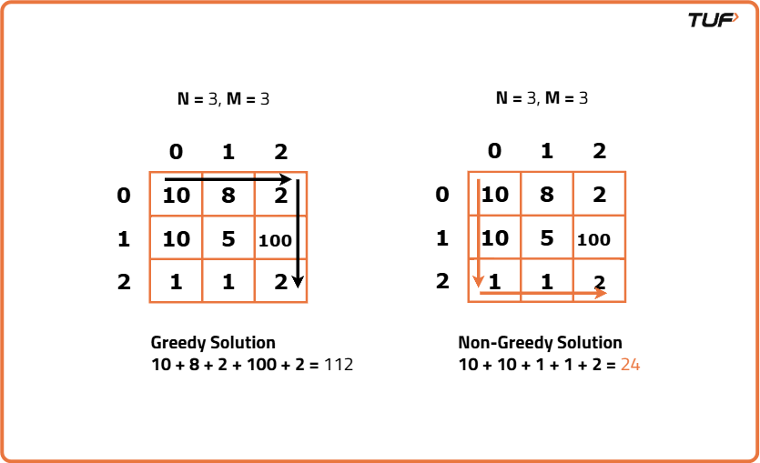
This is precisely where DP shines. By building a table of optimal solutions to subproblems, we ensure that at every step, our decision is based on the true optimal path up to that point.

Pattern 1: Unique Path Counting

Let's start with a classic path-counting problem.

Problem: A robot is on an m x n grid. It starts at the top-left corner (0, 0) and wants to reach the bottom-right corner (m-1, n-1). The robot can only move down or right at any point. How many unique paths are there?

To solve this with DP, we follow the same structured thinking as before:

1. Define the State: What is the subproblem we are solving? Let's define dp[i][j] as the number of unique paths from the start (0, 0) to the cell (i, j). Our final answer will be dp[m-1][n-1].

2. Find the Transition: How can we compute dp[i][j] from previous subproblems? Since the robot can only move down or right, to reach cell (i, j), it must have come from either the cell directly above, (i-1, j), or the cell directly to the left, (i, j-1). The total number of ways to reach (i, j) is simply the sum of the ways to reach those two prerequisite cells.

   This gives us our transition formula:

   $$dp[i][j]=dp[i-1][j]+dp[i][j-1]$$

3. Identify the Base Cases: How does the process start?

   • For any cell in the first row (i=0), there is only one way to get there: by moving right from the start. So, dp[0][j] = 1 for all j.
   • Similarly, for any cell in the first column (j=0), there is only one way to get there: by moving down from the start. So, dp[i][0] = 1 for all i.
   • The starting cell itself, dp[0][0], has one path (you are already there).

The following resource provides a clear, step-by-step explanation of this logic.

With this intuition, we can construct the tabulated solution. We create an m x n grid, initialize the base cases (the first row and column to all 1s), and then iterate through the rest of the grid, filling each cell using our transition formula.

Here is a TypeScript implementation that follows this logic directly.

function uniquePaths(m: number, n: number): number {
    // 1. Define the state: dp[i][j] is the number of paths to cell (i, j)
    // We create an m x n grid initialized to 0.
    const dp: number[][] = Array(m).fill(0).map(() => Array(n).fill(0));

    // 2. Initialize base cases
    // First row can only be reached by moving right.
    for (let j = 0; j < n; j++) {
        dp[0][j] = 1;
    }
    // First column can only be reached by moving down.
    for (let i = 0; i < m; i++) {
        dp[i][0] = 1;
    }

    // 3. Fill the table using the transition
    for (let i = 1; i < m; i++) {
        for (let j = 1; j < n; j++) {
            const pathsFromAbove = dp[i - 1][j];
            const pathsFromLeft = dp[i][j - 1];
            dp[i][j] = pathsFromAbove + pathsFromLeft;
        }
    }

    // The answer is the value in the bottom-right cell.
    return dp[m - 1][n - 1];
}

This approach has a time complexity of $O(m\times n)$ because we visit each cell of the grid once, and a space complexity of $O(m\times n)$ for the dp table.

Pattern 2: Minimum Cost Path

Now let's look at a variation. The movement rules are the same, but now the grid has values, and we want to find the path with the minimum total cost.

Problem: Given an m x n grid filled with non-negative numbers, find a path from the top-left (0,0) to the bottom-right (m-1, n-1) which minimizes the sum of all numbers along its path. You can only move either down or right at any point in time.

This problem is structurally identical to the last one, but the objective function changes from counting to minimizing.

1. Define the State: dp[i][j] will be the minimum cost to reach cell (i, j) from the start.

2. Find the Transition: Again, we can only arrive at (i, j) from (i-1, j) or (i, j-1). To ensure our path to (i, j) has the minimum possible cost, we must have come from the cell that had the cheaper path. So, we take the minimum of the costs to reach the preceding cells, and add the current cell's cost (grid[i][j]).

   This gives the transition:

   $$dp[i][j]=\text{grid}[i][j]+\min (dp[i-1][j],dp[i][j-1])$$

3. Identify the Base Cases:

   • The starting cell's cost is just its own value: dp[0][0] = grid[0][0].
   • For the first row, the cost accumulates from the left: dp[0][j] = dp[0][j-1] + grid[0][j].
   • For the first column, the cost accumulates from above: dp[i][0] = dp[i-1][0] + grid[i][0].

The following resource provides another excellent walkthrough for this pattern.

The TypeScript implementation directly mirrors this logic:

function minPathSum(grid: number[][]): number {
    const m = grid.length;
    const n = grid[0].length;

    // dp[i][j] will store the min path sum to reach (i, j)
    const dp: number[][] = Array(m).fill(0).map(() => Array(n).fill(0));

    // Base Case: Top-left corner
    dp[0][0] = grid[0][0];

    // Base Case: Fill first column
    for (let i = 1; i < m; i++) {
        dp[i][0] = dp[i - 1][0] + grid[i][0];
    }

    // Base Case: Fill first row
    for (let j = 1; j < n; j++) {
        dp[0][j] = dp[0][j - 1] + grid[0][j];
    }

    // Fill the rest of the table
    for (let i = 1; i < m; i++) {
        for (let j = 1; j < n; j++) {
            dp[i][j] = grid[i][j] + Math.min(dp[i - 1][j], dp[i][j - 1]);
        }
    }

    return dp[m - 1][n - 1];
}

Space Optimization for Grid DP

Just as we saw in our 1D "House Robber" problem, we should always check for space optimization opportunities. Look at the transition for both grid problems: to calculate dp[i][j], we only need values from the previous row (i-1) and the current row (i). We never need values from row i-2 or earlier.

This means we don't need to store the entire m x n grid. We can optimize the space complexity from $O(m\times n)$ to $O(n)$ (the width of the grid) by only keeping track of the previous row's dp values while we compute the current row.

The following video gives a great explanation of how to perform this optimization. While the instructor implements it by working from the bottom-right of the grid upwards, the principle is the same.

Conclusion

In this lesson, you've successfully extended your dynamic programming knowledge to 2D grids. You now have a powerful and reliable template for solving a whole new class of problems.

Key takeaways from today:

• Grid DP Pattern: Many problems involving paths on a grid can be solved with DP by building a table (or dp matrix) that stores the optimal solution to subproblems ending at each cell.
• State: The state dp[i][j] almost always represents the answer to the subproblem for the grid cell at (i, j).
• Transition: The transition formula for dp[i][j] is derived from the allowed moves. For "down and right" problems, it depends on the cells dp[i-1][j] (from above) and dp[i][j-1] (from the left).
• Counting vs. Optimization: The specific operation in the transition depends on the goal. For counting unique paths, you sum the possibilities (+). For finding a minimum/maximum cost, you select the best path (min() or max()).
• Space Optimization: Grid DP problems can often be space-optimized from $O(m\times n)$ to $O(\min (m,n))$ because each new row/column only depends on the previous one.

In our next lesson, we'll dive into another major category of DP problems: subset problems. You will learn to solve a subset-sum decision problem with zero-one dynamic programming, which involves making choices about including or excluding items from a set to meet a specific target.