Space Optimization in Dynamic Programming

Hello! In our last session, we transformed recursive, memoized dynamic programming solutions into iterative, bottom-up tabulated ones. This shift gave us more performant code that avoids recursion limits. You saw how tabulation involves building a dp table, often an array or a 2D grid, to store the results of subproblems.

Today, we'll take that one step further. One of the major advantages of the bottom-up approach is that it makes the data dependencies explicit. By analyzing how we fill the dp table, we can often spot a powerful optimization. This lesson focuses on a common interview expectation: reducing the memory footprint of your DP solution.

Your learning outcome is to reduce a dynamic program's memory when each state depends only on recent states. We'll see how to take solutions that seemingly require O(n) or O(m*n) space and shrink them to O(1) or O(n), respectively, without changing the time complexity.

From O(n) to O(1): The Constant Space Optimization

Let's revisit the Fibonacci sequence, which has the same structure as the "Climbing Stairs" problem. The tabulated solution from our previous lesson required an array of size n+1.

function fibTabulated(n: number): number {
    if (n <= 1) return n;
    
    // O(n) space
    const dp = new Array(n + 1);
    dp[0] = 0;
    dp[1] = 1;

    for (let i = 2; i <= n; i++) {
        // The transition:
        dp[i] = dp[i - 1] + dp[i - 2];
    }

    return dp[n];
}

Look closely at the transition: dp[i] = dp[i - 1] + dp[i - 2]. To calculate the value for dp[i], what information do we actually need? We only need the two immediately preceding values. We have no use for dp[i-3], dp[i-4], or any other earlier entries in the table. So why are we storing the entire array?

We don't have to. We can achieve the same result with just two variables holding the previous two values, reducing our space complexity from O(n) to O(1).

The instructor in the "take U forward" video series provides a fantastic walkthrough of this exact optimization. He shows how to evolve the O(n) tabulated solution into an O(1) space solution by thinking about the state you need at each step of the iteration.

This logic gives us the following highly optimized implementation.

The core idea is simple but powerful: identify the minimal state needed for the transition and only store that.

From O(m*n) to O(n): The Rolling Array Technique

This same principle applies to 2D dynamic programming. Consider a problem where you fill a grid, and the value for dp[i][j] depends only on cells in the same row (i) or the previous row (i-1).

This dependency pattern is very common in grid and string problems. For example, to calculate the green cell dp[i][j] below, you might only need the orange cells from the previous row or the current row. The red cells from two rows ago are no longer necessary.

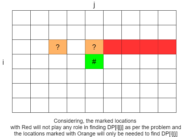
If we only need the previous row to compute the current one, why store the entire m x n grid? We can optimize by only keeping track of two rows at a time: the one we just finished computing (the "previous" row) and the one we are currently computing (the "current" row). After we finish the current row, it becomes the new "previous" row for the next iteration. This is called the rolling array technique.

Let's ground this with a clear textual explanation.

Worked Example: Unique Paths

Let's apply this to a classic problem: "Unique Paths" (LeetCode 62). A robot is on an m x n grid and wants to go from the top-left corner to the bottom-right corner. The robot can only move down or right. We need to find the number of unique paths.

A standard bottom-up DP solution involves creating an m x n grid where dp[i][j] stores the number of ways to reach cell (i, j). The number of ways to reach dp[i][j] is the sum of the ways to reach the cell above it (dp[i-1][j]) and the cell to its left (dp[i][j-1]). This gives a time and space complexity of O(m*n).

The NeetCode video on this problem provides one of the clearest explanations available.

Now, let's apply the space optimization. Since computing a row only requires the values from the row immediately above it, we don't need the whole grid. We can reduce the space to O(n) (the width of the grid). The video continues to explain exactly how to do this.

The video shows a very efficient implementation using a single row array. Another common way to implement this, which is sometimes conceptually easier, is to use two separate arrays, prevRow and currRow.

Here's what that would look like in TypeScript, based on the approach described in the resources.

function uniquePathsOptimized(m: number, n: number): number {
    // We only need to store one row's worth of data.
    // Let's use the smaller dimension for our DP array to save space.
    if (m < n) return uniquePathsOptimized(n, m); // ensure n is smaller
    
    let prevRow = new Array(n).fill(1);
    let currRow = new Array(n).fill(1);

    // Iterate through rows starting from the second row
    for (let i = 1; i < m; i++) {
        // Iterate through columns starting from the second column
        for (let j = 1; j < n; j++) {
            // The value is the sum of the one above (from prevRow)
            // and the one to the left (from currRow)
            currRow[j] = prevRow[j] + currRow[j-1];
        }
        // The current row now becomes the previous row for the next iteration.
        // We can swap or copy. Swapping is efficient if the language supports it well.
        // A simple copy is clear.
        prevRow = [...currRow];
    }
    
    // The result is the last element of the last computed row.
    return prevRow[n - 1];
}

This pattern—maintaining only the necessary previous state—is a hallmark of a polished DP solution.

Conclusion

You've now added a crucial optimization layer to your dynamic programming toolkit. Recognizing when a DP solution's space can be compressed is often what separates a good solution from a great one in an interview setting.

Here are the key takeaways:

• Analyze Dependencies: The key to space optimization is to analyze the transition formula in your bottom-up DP. What previous states are truly necessary to compute the current state?
• Constant Space O(1): For 1D DP problems like Fibonacci, if dp[i] only depends on a fixed number of predecessors (e.g., dp[i-1], dp[i-2]), you can replace the O(n) array with a few variables.
• Linear Space O(n) (Rolling Array): For 2D DP problems, if dp[i][j] only depends on the previous row (i-1) and the current row (i), you can reduce space from O(m*n) to O(min(m,n)) by only storing one or two rows at a time.

In our next lesson, we will begin exploring common DP patterns, starting with a fundamental one: solving a one-dimensional take-or-skip optimization problem. You'll find that the optimization techniques we've covered today are directly applicable to many of these patterns.