Conditional Totals and Counts with SUMIFS and COUNTIFS

Hello. In the previous lesson, you used IF to turn a business rule into a row-level label such as High Value, Over Budget, or On Target. Those labels make individual records easier to interpret. The next analyst task is to summarize them: How many high-value orders were there? What was their total revenue? How much did the West region sell in March?

This lesson introduces COUNTIFS and SUMIFS, which count or total records only when they meet the criteria you specify. They turn a transaction-level worksheet into a small, repeatable reporting tool.

---

Conditional summaries: choosing between a count and a total

A business question usually asks for one of two measures:

Question	Function	Example output
How many records meet these conditions?	COUNTIFS	42 orders
What is the total value of records meeting these conditions?	SUMIFS	$18,450 revenue

Both functions assess each row against a set of conditions. A row is included only when it meets every condition supplied. In other words, their logic is AND logic.

For example, consider an order dataset:

Order ID	Region	Salesperson	Revenue	Value Segment
ORD-1001	West	Priya	1,250	High Value
ORD-1002	East	Mateo	670	Standard
ORD-1003	West	Priya	1,000	High Value
ORD-1004	West	Chen	450	Standard

A manager might ask:

How many High Value orders were placed in the West region?

The first row qualifies: it is both West and High Value. The third row qualifies too. The other rows fail at least one condition, so they do not contribute to the result.

This is a different task from IF. IF classified one row at a time; COUNTIFS and SUMIFS summarize many rows at once.

---

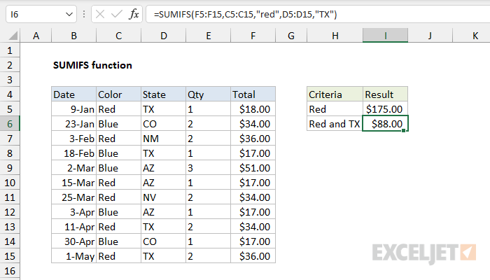
SUMIFS: total an amount that meets criteria

Use SUMIFS when the answer should be a numeric total, such as revenue, units sold, costs, profit, or hours.

Its structure is:

=SUMIFS(sum_range, criteria_range1, criteria1, [criteria_range2, criteria2], ...)

The order matters:

1. sum_range: the numbers to add.
2. criteria_range1: the column Excel should inspect for the first condition.
3. criteria1: what must be true in that column.
4. Further criteria range and criterion pairs, if needed.

The key distinction is that SUMIFS begins with the values to total. After that, every condition is entered as a range-and-criterion pair.

A two-condition revenue total

Suppose the worksheet uses these columns:

Column	Field
B	Region
D	Revenue
E	Value Segment

To calculate total revenue from High Value orders in the West region:

=SUMIFS($D$2:$D$101,$B$2:$B$101,"West",$E$2:$E$101,"High Value")

Read the formula in plain language:

Add revenue in D2:D101 when Region is West and Value Segment is High Value.

The dollar signs make the ranges absolute. This is helpful when you intend to copy the formula to adjacent cells in a summary table. The source data ranges should stay fixed.

Notice that text criteria are in quotation marks:

"West"
"High Value"

If the desired region is stored in a cell instead, use a cell reference without quotation marks. For example, if H2 contains West:

=SUMIFS($D$2:$D$101,$B$2:$B$101,$H$2,$E$2:$E$101,"High Value")

Using a criteria cell makes the summary more maintainable. Changing H2 from West to East updates the answer without requiring any formula editing.

Numeric conditions

Criteria can also test numbers. For example, to total revenue from orders worth at least 1,000:

=SUMIFS($D$2:$D$101,$D$2:$D$101,">=1000")

Here, the Revenue column has two roles:

• It is the sum range, containing the amounts to add.
• It is also the criteria range, because each revenue value must be at least 1,000.

This is valid. Excel checks each revenue amount, includes it if it meets the threshold, and then adds qualifying amounts.

For a reusable report, place the threshold in a labelled cell. If H3 contains 1000, write:

=SUMIFS($D$2:$D$101,$D$2:$D$101,">="&$H$3)

The ampersand joins two parts:

• ">=" is the comparison operator, written as text.
• $H$3 supplies the threshold value.

Excel turns these into one criterion, such as >=1000.

Common numeric criteria include:

Business rule	Criterion
Revenue exceeds 1,000	">1000"
Revenue is at least 1,000	">=1000"
Cost is below 500	"<500"
Discount is no more than 10%	"<=10%"
Status is not Cancelled	"<>Cancelled"

Be exact about the business boundary. “At least 1,000” requires ">=1000", not ">1000".

---

COUNTIFS: count qualifying records

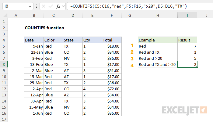
COUNTIFS uses the same range-and-criterion-pair pattern as SUMIFS, but it has no sum range. It counts qualifying rows rather than adding amounts.

=COUNTIFS(criteria_range1, criteria1, [criteria_range2, criteria2], ...)

For the earlier question, “How many High Value orders were placed in the West region?”, use:

=COUNTIFS($B$2:$B$101,"West",$E$2:$E$101,"High Value")

Read it as:

Count rows where Region is West and Value Segment is High Value.

The formula counts orders, not revenue. If three rows meet both tests, the answer is 3, regardless of the revenue amounts in those rows.

Count records using a number and text condition

Suppose you need to count West-region orders with revenue of at least 1,000:

=COUNTIFS($B$2:$B$101,"West",$D$2:$D$101,">=1000")

If the region and threshold are stored in H2 and H3, respectively:

=COUNTIFS($B$2:$B$101,$H$2,$D$2:$D$101,">="&$H$3)

This is a useful mini-reporting pattern:

Summary input	Example cell value
Selected region	H2: West
High-value threshold	H3: 1000

KPI	Formula
Number of qualifying orders	=COUNTIFS($B$2:$B$101,$H$2,$D$2:$D$101,">="&$H$3)
Revenue from qualifying orders	=SUMIFS($D$2:$D$101,$B$2:$B$101,$H$2,$D$2:$D$101,">="&$H$3)

The two formulas apply the same definition of a qualifying order. One answers how many, and the other answers how much.

---

Build formulas carefully: the most common errors

Conditional functions are powerful because they assess many rows quickly. That also makes small range or criterion mistakes consequential. Use this checklist when a result is unexpected.

Keep all ranges aligned

Every criteria range must cover the same rows as the sum range.

Correct:

=SUMIFS($D$2:$D$101,$B$2:$B$101,"West",$E$2:$E$101,"High Value")

Problematic:

=SUMIFS($D$2:$D$101,$B$2:$B$100,"West",$E$2:$E$101,"High Value")

The second formula uses a Region range that is one row shorter. Excel may return a #VALUE! error, or the formula structure may be difficult to audit. Select each range from the first data row through the same final data row.

Also exclude headers. If your records begin on row 2, begin every range at row 2.

Do not reverse SUMIFS arguments

This is correct:

=SUMIFS(sum_range,criteria_range,criterion)

For example:

=SUMIFS($D$2:$D$101,$B$2:$B$101,"West")

A frequent mistake is to place the sum range after the criteria pair, confusing SUMIFS with the older SUMIF function. Remember: with SUMIFS, the values to total come first.

Write criteria in the appropriate form

Use these rules:

• Direct text: "West"
• Direct numeric equality: 1000
• Direct numeric comparison: ">=1000"
• Cell containing text or a number: $H$2
• Comparison based on a cell: ">="&$H$3

This will not work correctly:

=COUNTIFS($D$2:$D$101,>=1000)

Excel needs the comparison operator and value to be interpreted together as a criterion:

=COUNTIFS($D$2:$D$101,">=1000")

Remember that all conditions must be true

This formula does not count every order that is either West or High Value:

=COUNTIFS($B$2:$B$101,"West",$E$2:$E$101,"High Value")

It counts only orders that are both West and High Value. Before building a formula, state the inclusion rule in a full sentence. If the request contains the word “or,” pause and clarify the intended logic rather than assuming that COUNTIFS or SUMIFS handles it directly.

---

Validate an analyst-style summary

Do not treat a plausible-looking number as proof that the formula is correct. A short validation routine makes your work defensible.

1. Filter the source table using the same criteria as the formula. For example, filter Region to West and Revenue to values of at least 1,000.
2. Check the visible row count against the COUNTIFS result.
3. Use the status bar or SUM on the visible Revenue values to compare with the SUMIFS result.
4. Inspect the formula bar to ensure each criteria range starts and ends on the same rows.
5. Test a boundary case. If the threshold is 1,000 and the definition says “at least,” confirm that an order worth exactly 1,000 is included.
6. Change a criteria cell deliberately. If the selected region changes from West to East, both count and total should update.

A concise explanation in a work setting could be:

I counted orders and summed revenue only for records in the selected region whose revenue met or exceeded the approved high-value threshold. I validated the formulas by applying equivalent table filters and reconciling the visible count and revenue total.

---

Key takeaways and next step

COUNTIFS and SUMIFS answer recurring business questions without manually filtering and calculating totals each time:

=COUNTIFS(criteria_range1, criteria1, ...)

=SUMIFS(sum_range, criteria_range1, criteria1, ...)

Remember:

• Use COUNTIFS for the number of qualifying records.
• Use SUMIFS for the total of a numeric measure among qualifying records.
• Each criteria range must match the size and position of the other ranges.
• SUMIFS places the sum range first; COUNTIFS does not use a sum range.
• Text and direct comparison conditions require quotation marks.
• Use criteria cells, absolute references, and & with comparison operators to build flexible summaries.
• Validate results by filtering the source data and checking boundary cases.

In the next module, you will begin preparing real-world Excel data for analysis by identifying missing values and formula errors, then choosing an appropriate treatment for each.