Ideal Op-Amp Characteristics

Hello! Welcome to your first lesson in the "Operational Amplifier Circuits" module. Given your background in Radiophysics and Electronics, this should be a great refresher and a solid foundation for the more advanced topics we'll tackle later.

Introduction

Approximate time to complete: 45 minutes

In this lesson, we will introduce the operational amplifier (op-amp), a cornerstone of analog electronics. Our goal is to understand the ideal op-amp model. This is a simplified, theoretical model that makes analyzing op-amp circuits much more manageable. We'll explore the key characteristics that define this ideal device. Understanding this model is crucial, as it provides the foundation for designing and analyzing the practical amplifier circuits we'll build in the upcoming lessons.

Let's begin by understanding what an op-amp is and why it's such a fundamental component.

What is an Operational Amplifier?

An operational amplifier is a high-gain voltage amplifier with a differential input and, typically, a single-ended output. Its name comes from its original use in analog computers to perform mathematical operations like addition, subtraction, integration, and differentiation.

To get a clear picture of its basic function and terminology, please watch the first part of the following video.

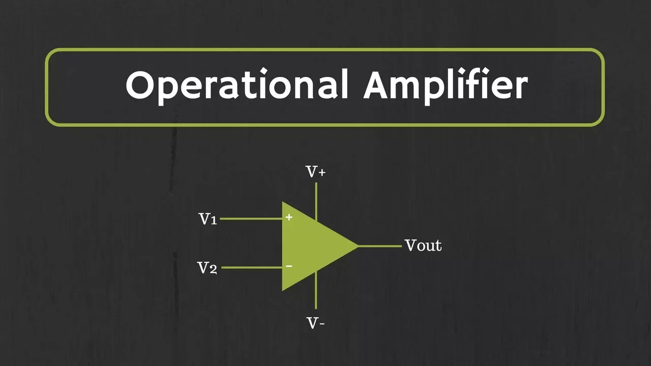
Watch from 00:19 to 04:12. Focus on:

• The circuit symbol for an op-amp.
• The roles of the non-inverting (+) and inverting (-) inputs.
• The basic output voltage equation: $V_{out}=A\times (V_{in,+}-V_{in,-})$.

As the video explains, the op-amp's primary job is to amplify the difference between the voltages at its two input terminals. The gain, represented by $A$, is called the open-loop gain because it's the gain without any feedback from the output back to the input.

The Ideal Model vs. Reality: Saturation

The open-loop gain $A$ of an op-amp is enormous—typically over 100,000. This has a significant real-world implication: even a tiny voltage difference between the inputs will, theoretically, create a massive output voltage.

For example, with a gain of $10^5$, a mere 1 mV difference at the input would result in a theoretical output of $10^{-3}V\times 10^5=100V$.

In practice, the output voltage can't exceed the power supply voltages used to bias the op-amp. This limitation is called saturation.

Please continue with the same video to understand this crucial concept.

Watch from 03:57 to 06:52. Pay attention to the voltage transfer curve, which visually explains how the output saturates.

This saturation effect is fundamental. When used without feedback (in an "open-loop" configuration), the op-amp acts more like a comparator, with its output swinging to either the positive or negative supply rail. To use it as a linear amplifier, we must introduce negative feedback, a topic we'll explore in the next lesson.

Characteristics of the Ideal Op-Amp

To simplify circuit analysis, engineers start with an ideal op-amp model. This model assumes a set of "perfect" characteristics. While no real op-amp is perfect, high-quality modern op-amps come remarkably close, making the ideal model incredibly useful for design.

The following video provides a clear, step-by-step breakdown of these ideal characteristics. We will go through them one by one.

---

1. Infinite Open-Loop Gain ($A_{OL}=\infty$)

An ideal op-amp has infinite voltage gain. This means it can amplify any infinitesimally small difference between its input terminals to produce a finite output voltage.

• Implication: This is the foundation for one of the "golden rules" of op-amp analysis with negative feedback: the circuit will work to keep the voltage difference between the two inputs at zero.
• Watch: from 00:40 to 01:46.

2. Infinite Input Resistance ($R_{in}=\infty$)

The resistance looking into the input terminals is infinite.

• Implication: An ideal op-amp draws zero current from the input source. It acts as a perfect voltmeter, sensing the input voltage without loading or disturbing the circuit it is connected to.
• Watch: from 01:46 to 02:52.

3. Zero Output Resistance ($R_{out}=0$)

The resistance in series with the internal voltage source of the op-amp is zero.

• Implication: The op-amp can supply any amount of current to the load, and its output voltage remains constant regardless of the load connected. It acts as a perfect voltage source.
• Watch: from 02:52 to 04:25.

4. Infinite Bandwidth

The op-amp can amplify signals of any frequency, from DC (0 Hz) to infinity, with the same constant gain.

• Implication: The amplification is independent of the signal's frequency.
• Watch: from 05:05 to 06:08.

5. Zero Output Offset Voltage

When the voltage difference between the input terminals is zero (i.e., $V_{in,+}=V_{in,-}$), the output voltage is exactly zero.

• Implication: The op-amp produces no output unless there's an actual difference at the input.
• Watch: from 04:00 to 05:26.

6. Infinite Common-Mode Rejection Ratio (CMRR)

The CMRR is a measure of how well the op-amp rejects signals that are common to both inputs (like noise). An infinite CMRR means the op-amp is a perfect differential amplifier, only amplifying the difference signal and completely ignoring the common-mode signal.

• Implication: The op-amp is perfectly immune to common-mode noise.
• Watch: from 05:49 to 08:04.

7. Infinite Slew Rate

The slew rate is the maximum rate of change of the output voltage. An infinite slew rate means the output voltage can change instantaneously in response to an instantaneous change at the input.

• Implication: The output can perfectly track fast-changing input signals without any distortion.
• Watch: from 07:44 to 09:28.

Summary: Ideal vs. Practical Op-Amp

Here is a table summarizing the characteristics of an ideal op-amp versus a typical, practical op-amp like the classic µA741. This helps put the ideal model into a real-world context.

Characteristic	Ideal Value	Practical Value (µA741)
Open-Loop Gain ($A_{OL}$)	$\infty$	$\approx 200,000$ V/V
Input Resistance ($R_{in}$)	$\infty$	$\approx 2$ M$\Omega$
Output Resistance ($R_{out}$)	$0$ $\Omega$	$\approx 75$ $\Omega$
Bandwidth	$\infty$	$\approx 1$ MHz
CMRR	$\infty$	$\approx 90$ dB
Slew Rate	$\infty$	$\approx 0.5$ V/$\mu$s
Output Offset Voltage	$0$ V	$\approx 1-5$ mV

For a final recap on this comparison, you can watch the last part of the ALL ABOUT ELECTRONICS video from 11:15 to 12:25.

Conclusion

In this lesson, we introduced the operational amplifier and defined the ideal op-amp model. This theoretical model is characterized by:

• Infinite open-loop gain
• Infinite input resistance
• Zero output resistance
• Infinite bandwidth
• Infinite CMRR and slew rate
• Zero offset voltage

The two most important takeaways for circuit analysis are infinite input resistance (zero input current) and infinite open-loop gain. When we apply negative feedback, these two properties give us the "golden rules" for analyzing op-amp circuits:

1. No current flows into the input terminals.
2. The voltage difference between the inverting and non-inverting inputs is zero ($V_{+}=V_{-}$).

In our next lesson, "Inverting and Non-Inverting Op-Amp Configurations," we will use these two rules to derive the gain equations for the most fundamental op-amp amplifier circuits. This will demonstrate just how powerful the ideal model is for practical design.