Compute-Bound vs. Memory-Bound Transformer Inference

Introduction

Welcome to Module 4: Compute Optimization. In the previous module, we developed a precise "napkin math" for the memory footprint of large language models. You learned how to account for every gigabyte of VRAM consumed by model weights, the KV cache, and activations. This answered the question of why LLMs are so memory-intensive.

Now, we shift our focus from memory capacity to time and speed. This module tackles the other side of the performance coin: why LLM inference can be slow, and what we can do about it. The foundational concept for all compute optimization is understanding the primary bottleneck at any given moment.

Today's lesson addresses this directly. Our learning outcome is to distinguish between compute-bound and memory-bandwidth-bound operations in transformer inference. Mastering this distinction is the first and most critical step in diagnosing performance issues and applying the correct optimization strategy. You will learn to move beyond treating the GPU as a black box and start reasoning about its fundamental architectural limits.

The Two Phases of Inference and Their Bottlenecks

As you know from our previous discussions, LLM inference isn't a single, monolithic process. It's composed of two distinct phases: prefill and decode. Intuitively, you might guess they have different performance characteristics, and you'd be right.

Let's start with a short, clear explanation of these two phases and why their computational profiles differ.

The key insight is that the nature of the work being done changes dramatically between processing the prompt and generating subsequent tokens.

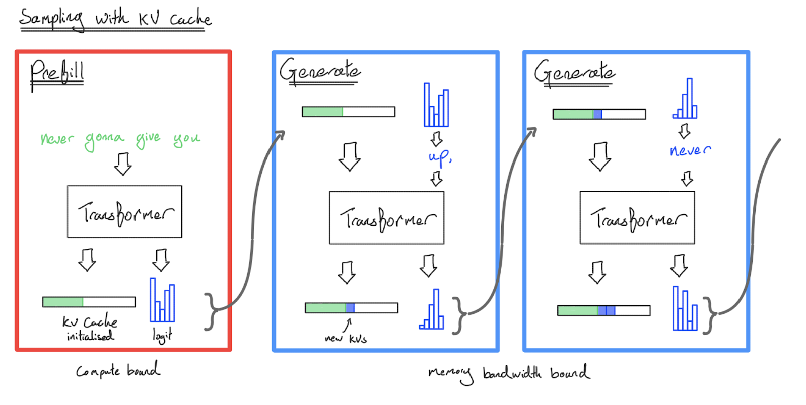
To formalize this, we need to define our terms. An operation is:

• Compute-bound when the total time is dominated by arithmetic calculations. The GPU's processing units (the CUDA cores and Tensor Cores) are the limiting factor, and they are running at or near 100% utilization. The speed is limited by the number of Floating Point Operations Per Second (FLOPS) the GPU can execute.
• Memory-bandwidth-bound when the total time is dominated by moving data (e.g., weights, activations, KV cache) between the GPU's main memory (HBM) and its on-chip processing units (SRAM/registers). The processing units are often idle, waiting for data to arrive. The speed is limited by the memory bandwidth (in GB/s) of the GPU.

To build a robust mental model, it's essential to understand the underlying hardware.

Quantifying the Bottleneck: The Roofline Model

The article you just read introduced the core concept for quantifying performance bottlenecks: arithmetic intensity. It is the ratio of compute operations to memory accesses for a given algorithm.

Arithmetic Intensity = Total FLOPs / Total Bytes Accessed

We can determine the bottleneck by comparing the arithmetic intensity of our algorithm to a similar ratio for our hardware.

This hardware ratio, often called the ops:byte ratio, tells us how many operations the GPU can perform in the time it takes to move one byte of data from HBM.

ops:byte Ratio = Peak FLOPS / Memory Bandwidth (GB/s)

Let's see a practical example of how to find this hardware ratio.

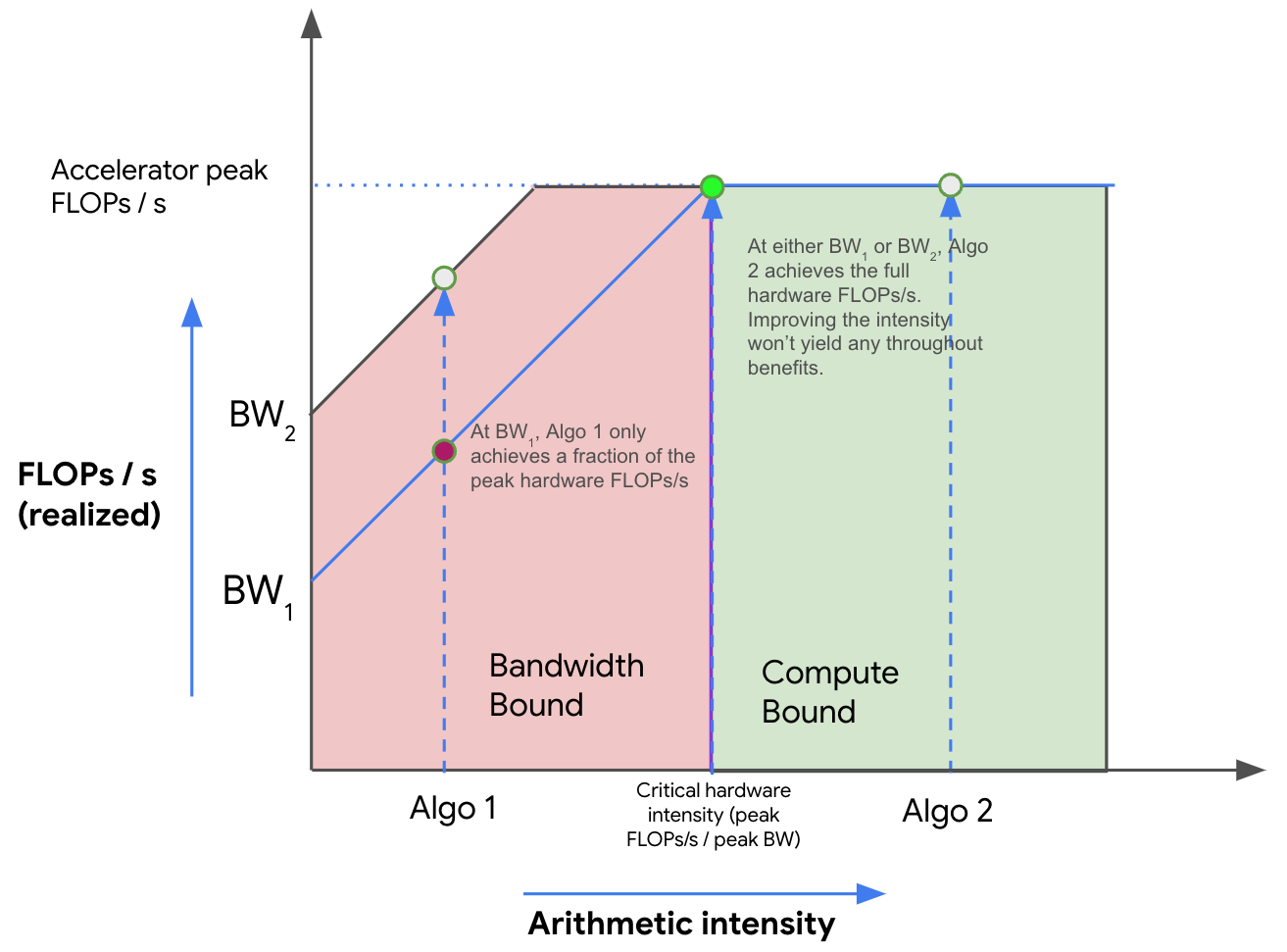
Now we have our decision rule:

• If Arithmetic Intensity < ops:byte Ratio, the operation is Memory-Bound. The algorithm performs too few computations for each byte it fetches, so the GPU spends most of its time waiting for data.
• If Arithmetic Intensity > ops:byte Ratio, the operation is Compute-Bound. The algorithm performs many computations for each byte, fully utilizing the GPU's arithmetic units.

This relationship is visually captured by the Roofline Model, a fundamental tool in performance engineering.

Analysis of Transformer Inference Phases

Let's apply this quantitative framework to the prefill and decode phases.

1. Prefill Phase (Compute-Bound)

During prefill, the model processes the entire input sequence of length $L$ in parallel. The self-attention mechanism, a dominant part of the computation, involves large matrix multiplications like $\mathbf{Q}{\mathbf{K}}^T$, where both matrices have dimensions related to $L$.

The number of compute operations scales roughly with $\mathcal{O}(L^{2}d+L{d}^2)$, while the memory accesses scale with $\mathcal{O}(L^{2}h+Ld+d^2)$.

For long input sequences, the sheer volume of parallelizable computation (large matrix-matrix products) outweighs the data movement costs, saturating the GPU's compute units.

2. Decode Phase (Memory-Bandwidth-Bound)

During autoregressive decoding, the situation is reversed. At each step, we generate a single token. The computation involves processing this one token's embeddings against the entire KV cache from all previous $L$ tokens.

• Compute: The amount of new computation is small, scaling with $\mathcal{O}(Ld)$. We are essentially performing matrix-vector multiplications.
• Memory Access: The amount of data moved is enormous. We must read the full $\mathbf{K}$ and $\mathbf{V}$ tensors (the KV cache) from slow HBM into the fast on-chip SRAM for every single token we generate. The size of the KV cache is $\mathcal{O}(Lnd)$, where $n$ is the number of layers.

This combination of low compute and high memory access results in a very low arithmetic intensity.

This fundamental difference is also highlighted in research on disaggregated serving systems.

Conclusion

In this lesson, you've learned to analyze LLM inference performance through the lens of its fundamental hardware limitations. This is a significant step up from simply measuring wall-clock time.

Key Takeaways:

• GPU operations are limited by one of two factors: compute performance (FLOPS) or memory bandwidth (GB/s).
• The Roofline Model provides the theoretical framework for determining the bottleneck by comparing an algorithm's arithmetic intensity to the hardware's ops:byte ratio.
• Transformer inference has two distinct phases with different bottlenecks:
  • Prefill involves large, parallel matrix multiplications, making it compute-bound.
  • Autoregressive Decoding involves small computations but requires reading the large KV cache from memory at every step, making it memory-bandwidth-bound.

This distinction is not just academic; it dictates our entire optimization strategy. Trying to optimize a memory-bound operation by making the math faster is pointless if the GPU is just waiting for data. Conversely, optimizing data movement for a compute-bound operation will yield no speedup.

Preview of the Next Lesson:

Now that you can identify the bottleneck, we will dive deeper into practical analysis. In the next lesson, you will learn to calculate the arithmetic intensity for key operations within the attention and FFN layers. We will then apply the roofline model concept to determine if a specific operation is compute- or memory-bound on a specific GPU, moving from the general (prefill/decode) to the specific (individual matrix multiplications, element-wise operations).