Scaling Model Capacity with Mixture of Experts (MoE)

Hello! Welcome to the final lesson in our module on Modern Language Model Architectures.

In our previous lessons, we've dissected the anatomy of models like LLaMA, exploring innovations like Rotary Positional Embeddings (RoPE), Grouped-Query Attention (GQA), and the SwiGLU activation function. Each of these improvements optimizes a specific component of the Transformer. Today, we zoom out to look at a paradigm-shifting architectural pattern that addresses the fundamental challenge of scaling: the Mixture of Experts (MoE).

As promised, we'll explore how MoE allows developers to build models with trillions of parameters while keeping the computational cost for inference surprisingly low. This is the key technology behind many of the latest state-of-the-art models, including Mistral's Mixtral, Google's Gemini, and is a core part of Meta's LLaMA 3 and 4 roadmaps. Our goal today is to understand how this seemingly magical feat is achieved.

1. The Core Idea: Scaling Parameters, Not Computation

The "scaling laws" in deep learning suggest that bigger models trained on more data perform better. However, simply making a dense model (like GPT-3 or LLaMA 2) bigger means every part of the model gets larger, and the computational cost (FLOPs) for every single token generation step increases. This path becomes economically and computationally unsustainable very quickly.

Mixture of Experts offers an alternative path: conditional computation. Instead of running the entire massive model for every token, what if we had a collection of smaller "expert" networks and intelligently selected only a few relevant ones to process each token?

This architecture consists of two main components:

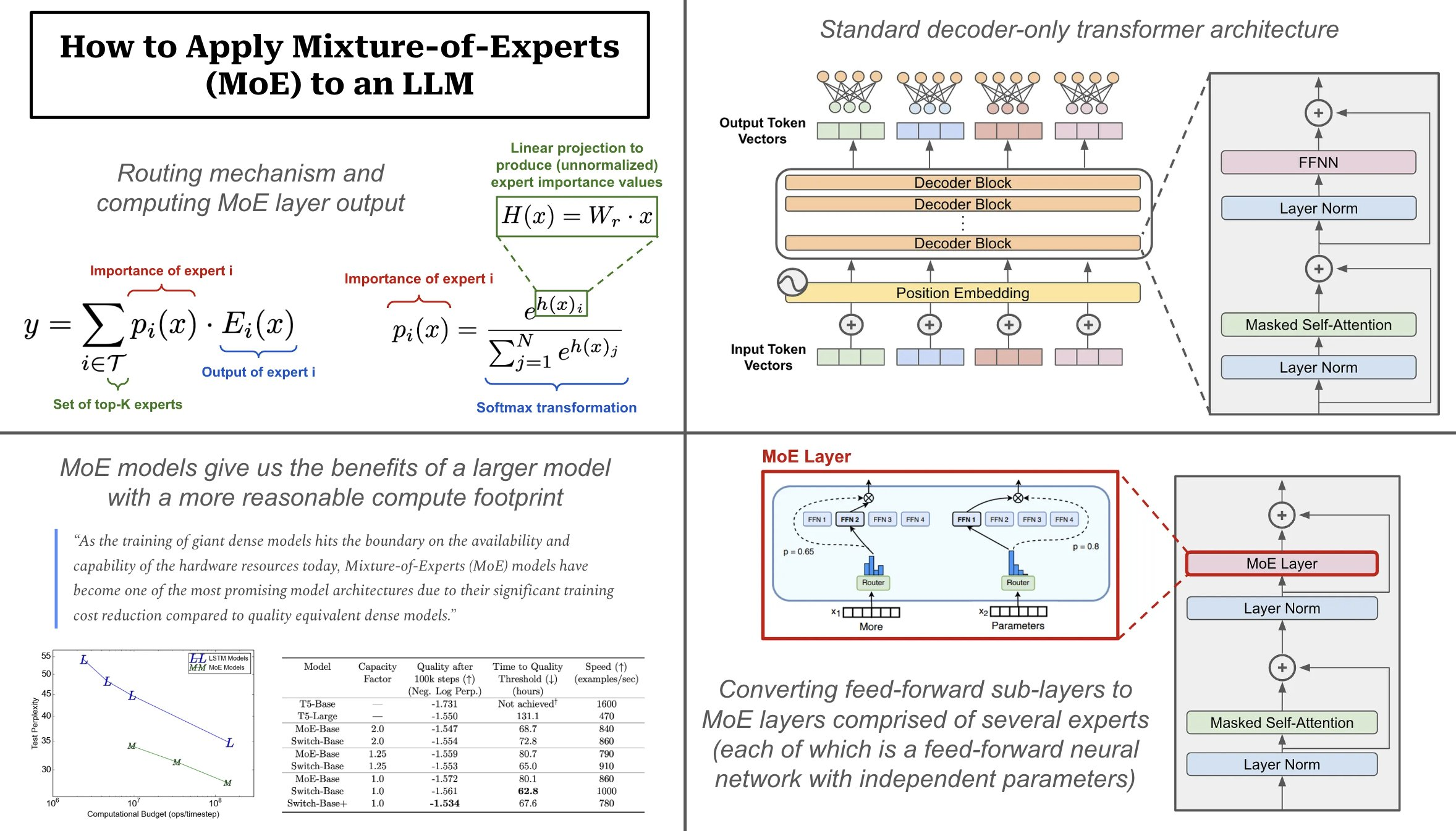
• Experts: These are specialized neural networks. In the context of Transformers, each expert is typically a standard Feed-Forward Network (FFN), just like the SwiGLU blocks we studied in the last lesson. A model might have anywhere from 8 to thousands of these experts.
• Router (or Gating Network): This is a small, trainable neural network that acts as a traffic controller. For each incoming token, the router decides which expert(s) are best suited to process it.

This design allows a model to have a huge number of total parameters (the sum of all experts and the rest of the model), but the number of active parameters used for any given token remains small and manageable.

2. From Dense to Sparse: The Evolution of MoE

The idea of MoE is not new; it originated in a 1991 paper for a simple classification task. The modern revival, however, introduced a crucial change that made it suitable for today's giant models: sparsity.

As the video explains, the key is the top-k gating mechanism:

1. The router network takes a token's embedding and computes a score for each expert, usually with a linear layer followed by a softmax function.
2. Instead of using all experts, it identifies the k experts with the highest scores. k is a small, fixed number, typically 1 or 2.
3. Only these k experts are activated and process the token. All other experts do no work.
4. The final output of the MoE layer is a weighted average of the outputs from the k active experts, with the weights being their softmax scores from the router.

This move from a dense, fully-connected system to a sparse, conditionally-activated one is what unlocks massive parameter counts without a corresponding explosion in computational cost.

Test your understanding!

Imagine a Transformer model where the FFN layer has been replaced by an MoE layer with 64 experts. The model uses top-2 routing. For a single input token, how many experts' FFNs are actually executed? How does the total number of parameters in the MoE layer compare to the number of active parameters for that token?

Show answer

Only 2 experts' FFNs are executed for that single token. The router selects the two with the highest scores, and the other 62 remain inactive.

The total number of parameters in the MoE layer includes the parameters of all 64 experts plus the router. The number of active parameters for that token only includes the parameters of the 2 selected experts, the router, and any other shared components. Therefore, the total parameter count is much larger than the active parameter count.

3. Key Challenges and Solutions in MoE Training

Implementing MoE effectively introduces several engineering and algorithmic challenges that don't exist in dense models. Successfully training an MoE model requires addressing them.

Challenge 1: Load Imbalance

A naive router might quickly learn to favor a few "popular" experts, sending most tokens their way. This is inefficient: the popular experts become computational bottlenecks, while the other experts are under-trained and useless. This is often called the "rich get richer" problem.

Solution: Auxiliary Load Balancing Loss
To counteract this, an additional loss term is added during training. This auxiliary loss penalizes the model if the distribution of tokens to experts is uneven. It incentivizes the router to spread the load as evenly as possible across all available experts, ensuring they all receive training signals.

The loss function for a batch of T tokens and N experts is often formulated as:

$$L_{\text{aux}}=\alpha \cdot N\sum _{i=1}^N{f}_i\cdot P_i$$

where:

• $f_i$ is the fraction of tokens in the batch dispatched to expert i.
• $P_i$ is the fraction of the router's probability mass allocated to expert i.
• $\alpha$ is a hyperparameter that controls the weight of this loss.

Challenge 2: Static Computation Graphs

Modern hardware and compilers (like those used in PyTorch and TensorFlow) are highly optimized for static tensor shapes. In MoE, the number of tokens routed to each expert is dynamic and unpredictable, which clashes with this requirement.

Solution: Expert Capacity
To solve this, a static buffer size, or capacity, is defined for each expert. This is the maximum number of tokens an expert can process in a given batch.

Expert Capacity = (Tokens per batch / Number of experts) × Capacity Factor

The Capacity Factor (e.g., 1.25) provides a small amount of extra buffer space. If an expert receives more tokens than its capacity, the "overflowing" tokens are dropped. Dropped tokens typically bypass the expert layer entirely, passing through the residual connection to the next layer. This ensures that tensor shapes remain static, but it comes at the cost of some tokens not getting the full computation.

As the video mentions, other techniques like using higher precision (float32) for the router calculations and carefully tuning initialization and dropout rates are also crucial for maintaining training stability in these massive, sparse models.

4. Do Experts Actually Specialize?

A natural question is whether these "experts" truly learn specialized functions. The answer is yes, but perhaps not in the way one might intuitively expect.

The key takeaway is that experts do specialize, but often on syntactic or grammatical patterns rather than high-level topics. For example, you might have an expert that becomes good at handling punctuation, another for proper nouns, or another for verbs in a specific tense. Due to the load-balancing loss, it's rare for an expert to specialize in a single topic (like "science" or "history"), as this would lead to it being under-utilized for other topics.

5. Modern MoE Architectures in Practice

Let's look at how these concepts are applied in some well-known models.

Recent popular open-source models have further refined this architecture:

• Mixtral 8x7B: Published by Mistral AI, this is a very strong open-source MoE model. It has 8 experts in total and uses top-2 routing (each token is processed by two experts). Although it's called "8x7B" (which would imply 56B parameters), its total parameter count is closer to 47B because only the FFN layers are experts; the attention and other parameters are shared. Its inference speed is comparable to a dense 13B model.
• DeepSeek-MoE & LLaMA 4: These models introduce the concept of a shared expert. In addition to the routed experts, there is one FFN that every token is sent to. This shared expert can learn common, universal knowledge, freeing up the other experts to become even more specialized.

Conclusion

Today we've demystified the Mixture of Experts architecture. It's not magic, but rather a clever application of conditional computation that allows for an elegant trade-off between model size and computational cost.

• Key Takeaways:
  • MoE replaces dense FFN layers with a large number of smaller "expert" FFNs.
  • A router network directs each token to a small subset of experts (typically 1 or 2) using top-k gating.
  • This sparsity allows models to have massive total parameter counts while keeping the active parameter count (and thus inference cost) low.
  • Training MoEs requires solving key challenges like load imbalance (with an auxiliary loss) and hardware constraints (with expert capacity).
  • Experts do specialize, often on syntactic or low-level semantic patterns, driven by the pressures of the learning objective and load balancing.

This lesson concludes our module on modern language model architectures. We have journeyed from the core Transformer to the specific optimizations in LLaMA and finally to the large-scale paradigm of MoE.

Preview of the Next Module:
Now that we have a deep understanding of how these models are built, the next logical question is: how do we control what they generate? How do we align their behavior with complex human instructions and preferences? Our next module, Reinforcement Learning Foundations, will lay the groundwork for answering this. We will start by formulating problems as Markov Decision Processes and exploring fundamental algorithms like value and policy iteration, which are the building blocks for advanced techniques like Reinforcement Learning from Human Feedback (RLHF).