Exploring BERT and Its Variants

Hello! Welcome to the first lesson in our module on Modern Language Model Architectures.

In the previous module, we established the "why" and "what" of transfer learning in NLP. You learned about the pre-train/fine-tune paradigm, where a model first learns general language understanding on a massive unlabeled corpus and is then adapted for specific downstream tasks. Today, we dive into the architecture of the model that truly popularized this paradigm: BERT.

Our learning outcome for this lesson is to analyze the architecture of BERT and its variants (RoBERTa, ALBERT). We will dissect the components that make BERT so effective for language understanding tasks and then explore how subsequent models built upon its foundation, either by optimizing its training or by making it more efficient.

1. BERT: Bidirectional Encoder Representations from Transformers

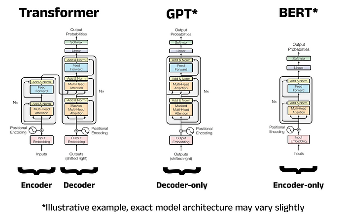
BERT's name tells you almost everything you need to know. It uses the Encoder part of the Transformer architecture to generate Bidirectional Representations. This design was a deliberate departure from the full encoder-decoder structure of the original Transformer and the decoder-only structure of models like GPT.

The central idea behind BERT is to create a model whose sole purpose is to understand text deeply, rather than generate it. This makes it a powerful feature extractor for a wide array of NLP tasks.

1.1 Core Architectural Components

BERT's architecture consists of a stack of Transformer encoder blocks. The popular BERT-base model uses 12 of these blocks, while BERT-large uses 24. Since you're familiar with the Transformer encoder from a previous module, we'll focus on what makes BERT's usage unique.

Bidirectionality through Self-Attention
The key feature of the encoder is its self-attention mechanism. Unlike RNNs, which process text sequentially, or GPT's masked self-attention, which only looks at past tokens, the self-attention in BERT's encoders allows every token to attend to every other token in the sequence simultaneously. This is what makes BERT truly bidirectional. It builds a representation of each word based on the entire context, both left and right.

1.2 Input Representation: More Than Just Words

A crucial part of BERT's design is how it formats its input. The final input embedding for each token is the sum of three distinct embeddings:

1. Token Embeddings: These are learned embeddings for sub-word units from the vocabulary, generated using a method called WordPiece tokenization. This allows the model to handle out-of-vocabulary words and a large vocabulary efficiently.
2. Segment Embeddings: These are used to distinguish between different sentences in the input. For example, in a question-answering task, sentence A could be the question and sentence B the context paragraph. All tokens in sentence A get one learned embedding (E_A), and all tokens in sentence B get another (E_B).
3. Positional Embeddings: Since the self-attention mechanism itself has no sense of order, these embeddings are added to give the model information about the position of each token in the sequence. Unlike the original Transformer that used sinusoidal functions, BERT uses learned positional embeddings.

1.3 Special Tokens and Pre-training Objectives

BERT's architecture is intrinsically linked to its two pre-training objectives, which we touched upon in the last module. These tasks force the model to learn the rich representations we need for downstream applications.

Let's summarize the key points:

1. Masked Language Modeling (MLM):

   • Objective: Predict randomly masked words in a sentence. This is the "fill-in-the-blanks" game.
   • Purpose: This task forces the model to learn deep contextual understanding. To predict a masked word correctly, the model must leverage the bidirectional context. This trains the token-level representations.
   • Mechanism: During pre-training, 15% of tokens are masked. The model's output for these masked positions is fed into a classifier to predict the original word. The loss is calculated only on these masked predictions.

2. Next Sentence Prediction (NSP):

   • Objective: Given two sentences, A and B, predict whether B is the actual sentence that follows A in the original text.
   • Purpose: This task forces the model to learn relationships between sentences, which is crucial for tasks like Question Answering and Natural Language Inference. This task specifically trains the [CLS] token's representation.
   • Mechanism: A special [CLS] (classification) token is prepended to every input sequence. The final hidden state corresponding to this token is used as the aggregate sequence representation for classification tasks. During NSP training, this [CLS] representation is fed into a simple binary classifier to predict IsNext or NotNext.

Additionally, a [SEP] (separator) token is used to explicitly mark the boundary between sentences.

The combination of these elements—MLM for token-level understanding and NSP for sentence-level understanding—is what made BERT a powerful, general-purpose pre-trained model.

Test your understanding!

You are tasked with building a model to determine if two questions from a forum are duplicates of each other (a sentence-pair classification task). Using a fine-tuned BERT model, which part of the final output would you use to make the classification decision, and why?

Show answer

You would use the final hidden-state vector corresponding to the special [CLS] token.

Reasoning: The [CLS] token is specifically designed and pre-trained (via the Next Sentence Prediction task) to aggregate the meaning of the entire input sequence (in this case, the two questions) into a single vector suitable for classification tasks. You would pass this single vector into a classifier (e.g., a linear layer followed by a softmax) to get your final prediction (duplicate or not duplicate).

2. RoBERTa: A Robustly Optimized BERT Approach

Soon after BERT was released, researchers at Facebook AI investigated whether it could be improved. They found that some of BERT's original design choices were sub-optimal and that significant performance gains could be achieved by simply changing the training strategy, without altering the core architecture. The result was RoBERTa.

Fundamentally, RoBERTa has the same architecture as BERT. The "analysis" of this variant is a crucial lesson in AI research: sometimes, the recipe is more important than the ingredients.

Here is a breakdown of RoBERTa's key optimizations:

Feature	BERT	RoBERTa	Impact
Pre-training Task	MLM + NSP	MLM only	The RoBERTa team found NSP was not very useful and removing it slightly improved performance.
Masking Strategy	Static Masking: Data is masked once and for all.	Dynamic Masking: Mask pattern is regenerated for each sequence every time it's fed to the model.	Provides more variety to the model during training, making it more robust.
Training Data	16GB (BooksCorpus, Wikipedia)	160GB (added CC-News, OpenWebText, Stories)	More data leads to better generalization.
Batch Size	256	8,000	Larger batches stabilize training and can improve final performance.
Tokenizer	WordPiece	Byte-level BPE	A slightly different sub-word tokenization scheme.

The takeaway from RoBERTa is profound: meticulous tuning of the pre-training process can yield results that are as significant as major architectural innovations.

3. ALBERT: A Lite BERT for Self-supervised Learning

While RoBERTa focused on maximizing performance, another variant, ALBERT, tackled a different problem: the enormous size of BERT models. BERT-large has 340 million parameters, making it difficult to train and deploy in resource-constrained environments. ALBERT introduced several clever architectural changes to drastically reduce the parameter count while maintaining competitive performance.

Here are ALBERT's two main architectural innovations:

1. Factorized Embedding Parameterization: In BERT, the WordPiece embedding size $E$ is tied to the hidden layer size $H$ (e.g., 768). This means the vocabulary embedding matrix is very large: Vocabulary Size (V) x Hidden Size (H). ALBERT decouples this by factorizing the embedding matrix into two smaller matrices. It first projects the one-hot vectors into a much lower-dimensional embedding space of size $E$ (e.g., 128) and then projects that into the hidden space $H$. This reduces the embedding parameters from $O(V\times H)$ to $O(V\times E+E\times H)$, which is a significant saving when $E\ll H$.

2. Cross-Layer Parameter Sharing: This is the most aggressive parameter reduction technique. Instead of each of the 12 or 24 Transformer blocks having its own unique set of weights, ALBERT shares the same block of weights across all layers. This is analogous to a recurrent neural network unrolled in time, but applied to the depth of the network. This single change reduces the number of parameters for the encoder blocks by an order of magnitude.

Finally, ALBERT also replaced the NSP task with a more challenging one called Sentence-Order Prediction (SOP). Instead of predicting if a second sentence is random, SOP asks the model to predict if two consecutive sentences from the same document have been swapped. This forces the model to learn about finer-grained coherence and discourse structure.

Conclusion

In this lesson, we deconstructed the architecture of BERT, the model that defined an era in NLP. You've seen how its encoder-only, bidirectional design is tailored for language understanding, and how its pre-training objectives (MLM and NSP) and unique input format work together to create powerful, general-purpose representations.

We then analyzed its most influential variants:

• Key Takeaways:
  • BERT introduced a powerful paradigm for pre-training deep bidirectional representations for a wide range of NLP tasks. Its architecture is built around the Transformer encoder.
  • RoBERTa demonstrated that the pre-training recipe (more data, dynamic masking, larger batches, no NSP) was just as important as the architecture itself, achieving superior performance with the same model structure.
  • ALBERT showed how to make these models more parameter-efficient through clever architectural changes like factorized embeddings and cross-layer parameter sharing, making large models more accessible.

Preview of the Next Lesson:
We've now thoroughly examined the bidirectional, encoder-only family of models. In our next lesson, we will turn our attention to the other side of the Transformer world: the autoregressive, decoder-only models. We will analyze the architecture of the GPT series and understand the critical role of causal attention in making them the powerful text generators they are today.