LLM Serving Stack: From Request to Token

Hello and welcome to the course! I'm excited to guide you on your journey from AI Engineer to AI Systems Engineer. Given your extensive background in computer science, we'll be able to move quickly and focus on bridging the specific gap you've identified: the low-level mechanics of running large language models efficiently in production.

This first module is all about building a solid "request-to-token" mental model. Before we dive into writing code, optimizing memory, or scaling across hardware, it's crucial to have a clear, high-level picture of what happens inside an LLM serving system.

Today's lesson, the very first in our course, is designed to give you exactly that. Our goal is to trace the full lifecycle of an HTTP request to its final token output. We'll do this by examining a state-of-the-art serving engine, vLLM, and learning about the tools used to observe and measure its behavior. By the end of this lesson, you'll have a conceptual map that we will flesh out with practical, hands-on implementation in the lessons to come.

The Conceptual Journey of a Prompt

When you send a prompt to a service like ChatGPT or a self-hosted model, it kicks off a multi-stage process optimized for speed and efficiency. To understand this journey, we'll use a high-performance open-source inference engine, vLLM, as our primary example.

To start, let's build a visual mental picture of this process. The following video provides an excellent, accessible walkthrough of how a production-level system like vLLM handles incoming prompts.

How the VLLM inference engine works?

This video, 'How the VLLM inference engine works?', provides a fantastic visual explanation of the core concepts we'll discuss. It will help you build a strong mental map of the entire process.

Please watch the following segments: Introduction (00:00 - 04:56): Pay attention to the core problem statement: what happens to a prompt as it goes through an inference engine? Tokenization (17:54 - 20:39): This covers the first fundamental step of converting text to numbers that the model can understand. The Waiting Queue (20:39 - 22:08): Focus on the introduction of the 'waiting queue' and the distinction between 'prefilling' and 'decoding' requests. Prefill vs. Decode & The KV Cache (22:08 - 27:57): This is a critical section. Concentrate on understanding why the KV cache is essential and how it leads to two distinct computational stages: prefill and decode.

Based on the video, let's formalize the key stages of the request-to-token lifecycle:

Request Arrival & Queueing: An HTTP request containing the prompt arrives at the API server. The engine doesn't process it immediately; instead, it places the request into a waiting queue.
Tokenization: The raw text prompt is converted into a sequence of numerical token IDs using a tokenizer specific to the model. From this point on, the engine works exclusively with these IDs.
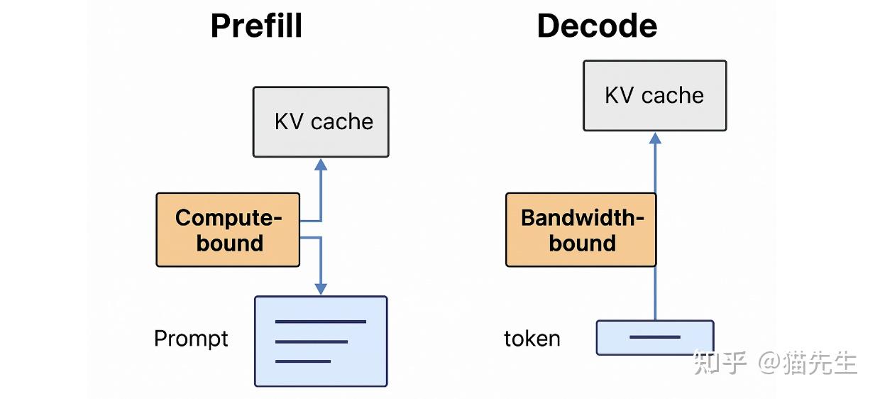
Scheduling: A scheduler decides which requests from the waiting queue to process in the next computation step. It prioritizes requests that are already being processed (running requests) over new ones. This is key to achieving high throughput.
Prefill (First Token Generation): This is the forward pass for the entire prompt. All prompt tokens are processed in a large, parallel batch to compute their corresponding Key and Value (KV) vectors. This initial computation is intensive and is typically compute-bound. The resulting KV vectors are stored in what's called the KV Cache. At the end of this stage, the very first output token is generated.
Decoding (Autoregressive Generation): For every subsequent token, the model performs a forward pass using only the single previously generated token. It re-uses the KV vectors for all preceding tokens from the KV Cache, avoiding costly re-computation. This stage is typically memory-bandwidth-bound because the main bottleneck is reading the large model weights and the KV cache from GPU memory.
Detokenization & Streaming: As each new token ID is generated during the decoding phase, it's converted back into text and sent back to the client. This is why you see the response appearing word by word.

The following diagrams provide a visual summary of these concepts.

LLM Inference: Prefill vs. Decode Bottlenecks — This diagram illustrates the different performance characteristics of the Prefill and Decode stages. Prefill is limited by raw compute power, while Decode is limited by how fast data can be read from GPU memory (memory bandwidth).

LLM Request Lifecycle: Preempted Decode Intervals — This diagram from the vLLM documentation shows the timeline of a request, highlighting key events from arrival to token generation and introducing metrics like Time-To-First-Token (TTFT) and Inter-Token Latency (ITL).

From Conceptual to Concrete: Tracing the vLLM Stack

Now that we have the conceptual framework, let's ground it in the actual architecture of vLLM. You don't need to memorize every detail, but seeing how these concepts map to a real system is the first step toward true systems engineering.

The following reading from the official vLLM blog provides a detailed anatomy of the engine.

Inside vLLM: Anatomy of a High-Throughput LLM Inference System

This blog post, 'Inside vLLM: Anatomy of a High-Throughput LLM Inference System', gives us an under-the-hood look. It connects the concepts from the video to the actual software components.

Focus on these parts to see how our conceptual model maps to vLLM's implementation: Generate function: Read the sections 'Generate function' and the subsequent 'Engine loop' diagram. This traces how a request is tokenized, added to the scheduler's queue, and processed in a step() loop. Scheduler: Read the 'Scheduler' section. Note how it explicitly handles 'Prefill' and 'Decode' requests as two different workload types, prioritizing decoding. Full request lifecycle (putting it all together): Skim the final section, 'So, putting it all together, here’s the full request lifecycle!'. It provides a step-by-step trace of a curl request through the entire distributed system, from the API server to the engine core and back. This directly addresses today's learning outcome.

Instrumenting the Stack: How to Measure the Lifecycle

Tracing the lifecycle isn't just a conceptual exercise. As a systems engineer, your job is to measure, analyze, and optimize it. To do this, you need tools to "instrument" the serving stack.

Instrumentation can happen at different levels:

Black-box (End-to-End): Measuring performance from the client's perspective.
White-box (Internal): Looking inside the server to see where time is being spent.

A crucial part of black-box analysis is benchmarking. Simply sending one request with curl isn't enough to understand how a system performs under load. Specialized tools are needed to simulate realistic traffic and measure key performance indicators (KPIs).

The following video from NVIDIA provides an excellent overview of production-grade LLM benchmarking.

AI Perf benchmarking - Dynamo and other LLM endpoints

This video, 'AI Perf benchmarking - Dynamo and other LLM endpoints', introduces a professional tool for benchmarking and explains the critical metrics we use to evaluate LLM inference performance.

Watch these segments to understand how we measure the performance of our request-to-token lifecycle: Simple Benchmarking Command (05:39 - 12:46): Focus on the command arguments (concurrency, request-count, ISL/OSL) and the output metrics. Pay close attention to the definitions of Time-to-First-Token (TTFT) and request latency. Think about how TTFT relates to the 'prefill' phase and how the overall tokens-per-second relates to the 'decode' phase. Trace-based Benchmarking (21:09 - 28:05): Understand why replaying real-world traffic traces (like the Moon Cake dataset) is more realistic than using synthetic, fixed-length prompts. This is especially important for evaluating optimizations like the KV cache. Goodput Analysis (30:32 - 33:22): This introduces the concept of a Service Level Agreement (SLA) and 'goodput'—the percentage of requests that actually meet your performance targets. This is a critical metric for production readiness.

Diving Deeper with Profiling

Benchmarking gives us the "what" (e.g., "TTFT is 500ms"), but it doesn't always tell us the "why." To understand the internal performance, we use profilers. A profiler attaches to the running code and records the time spent in each function or even each low-level GPU operation.

In future lessons, we will use profilers extensively. For now, it's important to know that these tools exist and how to enable them. The vLLM documentation provides clear instructions for using standard tools like PyTorch Profiler and NVIDIA Nsight Systems.

Profiling vLLM

This documentation on 'Profiling vLLM' shows how to enable built-in profilers to get a fine-grained view of the engine's internal operations. We will use these techniques in later lessons.

Read the section 'Profile with PyTorch Profiler', including the sub-section 'OpenAI Server'. You don't need to run the commands now, but understand that you can start the server with a special flag (--profiler-config) and then use API calls to start and stop the profiling process. This is a powerful way to instrument a live serving stack.

By combining black-box benchmarking with white-box profiling, we can get a complete picture of the request-to-token lifecycle, identify bottlenecks, and validate the impact of our optimizations.

Conclusion

In this lesson, we established the foundational mental model for our entire course. We have traced the journey of a prompt from a simple HTTP request to a stream of tokens, a process that underpins every modern LLM application.

Key Takeaways:

The LLM inference lifecycle consists of distinct stages: queueing, tokenization, scheduling, prefill, and decoding.
The prefill stage processes the entire prompt at once and is typically compute-bound. It is the primary determinant of the Time-To-First-Token (TTFT).
The decode stage generates subsequent tokens one-by-one, reusing the KV Cache, and is typically memory-bandwidth-bound. Its speed determines the Inter-Token Latency (ITL) or tokens-per-second.
High-throughput serving engines like vLLM use techniques like continuous batching and paged attention to efficiently manage the scheduler and KV Cache.
We can instrument this lifecycle using benchmarking tools (like AIPerf) to measure end-to-end performance (TTFT, throughput) and profilers (like PyTorch Profiler) to analyze internal operations.

Preview of the Next Lesson:

We've now seen the lifecycle from a high level using vLLM. In the next lesson, we will get closer to the code. We will map the conceptual stages of inference (tokenization, prefill, decode) to the corresponding function calls in a Hugging Face Transformers generate pipeline. This will bridge the gap between our high-level mental model and the underlying implementation.