When Speculative Decoding Improves Performance

Welcome back. In the previous lesson, FlashAttention showed how an inference or training kernel can become faster by moving less data through high-bandwidth memory, even while doing essentially the same mathematical work. Speculative decoding applies the same performance instinct at a different level: during autoregressive decode, the target model often reloads enormous weights to produce just one token, leaving compute capacity underused.

This lesson develops a quantitative answer to a systems question: when does it pay to spend work on drafting and verifying several possible tokens rather than decoding one token at a time? You will calculate the expected tokens produced per target-model step, translate that into latency speedup, and adjust the ideal calculation for real verification and scheduling costs.

---

The basic bargain: extra compute for fewer serial target steps

Ordinary autoregressive decoding is strictly serial. To generate each new token, the target model reads its weights and the relevant KV cache, runs a forward pass, samples one token, and repeats. At low concurrency, this is commonly memory-bandwidth-bound: moving weights through the GPU memory hierarchy takes longer than using the available arithmetic units.

Speculative decoding inserts a cheap draft mechanism:

1. A draft model proposes $\gamma$ future tokens sequentially.
2. The target model evaluates the proposed continuation in a single verification pass, producing target probabilities at every proposed position.
3. The system accepts the initial run of draft tokens that passes the target’s acceptance rule.
4. At the first rejection, later draft tokens are discarded and a corrected token is sampled from the target-derived distribution. If every draft token is accepted, the target can emit one additional “bonus” token.

Thus, one speculative iteration always emits at least one token and can emit up to $\gamma+1$ tokens.

{"type":"image","url":"https://developer-blogs.nvidia.com/wp-content/uploads/2024/12/speculative-decoding-workflow.jpg","caption":"A small draft model proposes several continuation tokens, while the large target model verifies their positions together. When a proposal is rejected, the remaining draft suffix is discarded and generation resumes from a target-consistent token.","isV2":true,"blockId":"40fa5cee-e73c-4cd4-b864-76fc26ac3b59","lessonId":"ae310d0c-753b-417f-8134-b876b44847c4"}

The crucial point is that verification is not free in terms of total GPU work. The target model evaluates several positions rather than one. It can nevertheless be close to the latency of a one-token decode step when the baseline is memory-bound: the target weights are fetched once and reused across more token positions, filling otherwise idle compute capacity.

For a visual explanation of this mechanism and why it is attractive specifically during memory-bound decode, watch the following two excerpts.

{"type":"video","title":"Speculative Decoding: The ONLY Video You Need to Speed Up Inference","learning_duration":219,"video_id":"_hEGvCwHyH8","par_intro":"“Speculative Decoding: The ONLY Video You Need to Speed Up Inference” by Cloud Codes gives a compact visual account of draft generation, parallel target verification, and the three quantities that determine the payoff.","par_directions":"Watch <span data-type=\"resource_video_timerange\" data-resource-subitem-id=\"0491fac1\" data-range-start=\"198\" data-range-end=\"360\">the core workflow</span>, focusing on why scoring several positions can reuse one target-model weight pass and why rejection still guarantees progress. Then watch <span data-type=\"resource_video_timerange\" data-resource-subitem-id=\"7c370c99\" data-range-start=\"402\" data-range-end=\"459\">the cost tradeoff</span>, which introduces draft quality, draft expense, and proposal length as coupled variables.","video_duration":1215,"isV2":true,"blockId":"acf3dd1a-9fe8-4807-a166-f7b0d32ea125","lessonId":"ae310d0c-753b-417f-8134-b876b44847c4"}

A caveat on “lossless” performance claims: with correct speculative sampling, the output distribution matches sampling directly from the target model under the same sampling transformations. It does not generally mean an independently seeded speculative request will generate the same literal sampled string as a baseline request. The guarantee comes from acceptance-rejection correction, not from treating a draft token as automatically correct whenever it matches a greedy choice.

---

Acceptance rate is the variable that turns guesses into useful work

Let $\alpha$ be the probability that an individual proposed token is accepted, averaged over the workload. This is the draft acceptance rate.

For distribution-preserving speculative sampling, a proposed token $x$ drawn from the draft distribution $q$ is accepted with probability

$$\min \left( 1, \frac{p(x)}{q(x)} \right)$$

where $p$ is the target distribution at that position. If the target assigns at least as much probability to the proposed token as the draft, it is accepted. Otherwise, it is accepted probabilistically. On rejection, sampling from a corrected residual distribution removes the draft’s bias.

So $\alpha$ is not merely “the fraction of tokens whose greedy IDs match.” It measures the probability of acceptance under the actual sampling and rejection policy. It depends on:

• the draft-target pair;
• the prompt and output domain;
• temperature, top-$p$, top-$k$, and other sampling transforms;
• decoding position and context length;
• the proposal method, such as a separate draft model, a draft head, or prompt lookup.

A coding-editing workload, for example, may have repeated or predictable text and yield much higher acceptance than open-ended creative writing. A single acceptance number reported by a model provider is therefore not enough for capacity planning.

Here is the mathematical foundation from the original speculative decoding paper.

{"type":"reading","par_intro":"Read Sections 2 and 3 of this arXiv paper for the original distribution-preserving algorithm and its ideal wall-time model. The goal is not to memorize the rejection-sampling proof, but to understand what the acceptance rate and draft-cost coefficient mean operationally.","par_directions":"In Section 2.1, “Overview” (p. 2), read <span data-type=\"resource_reading_textrange\" data-resource-subitem-id=\"9a63003c\" data-range-start=\"That way, each parallel run of the target model\" data-range-end=\"depending on how well Mq approximates Mp.\">the workflow summary</span> and notice the lower bound of one token and upper bound of \\(\\gamma+1\\) tokens per target pass.\n\nIn Section 3.1, “Number of Generated Tokens” (p. 3), follow <span data-type=\"resource_reading_textrange\" data-resource-subitem-id=\"9cbe6910\" data-range-start=\"capped geometric variable, with success probability\" data-range-end=\"See Figure 2.\">the expectation argument</span>. Focus on why each successive proposed token contributes only if all preceding proposals were accepted.\n\nThen read Section 3.3, “Walltime Improvement” (p. 3), especially <span data-type=\"resource_reading_textrange\" data-resource-subitem-id=\"40ed7a3c\" data-range-start=\"To get the total walltime improvement, we now consider\" data-range-end=\"often negligibly close to 0.\">the cost model</span>. Section 3.4 explains why lower wall-clock latency can still mean more total arithmetic operations.\n\nFinally, read Section 3.5, “Choosing \\(\\gamma\\)” (p. 4). Its opening discussion begins with <span data-type=\"resource_reading_textrange\" data-resource-subitem-id=\"9e90c7dd\" data-range-start=\"the number of memory accesses can go down with our method.\" data-range-end=\"according to Equation (1).\">the memory-traffic interpretation</span>; then examine how the proposed-token count is selected numerically rather than assumed to be universally optimal.","learning_duration":"18 minutes","url":"https://arxiv.org/pdf/2211.17192","title":"arXiv:2211.17192v2 [cs.LG] 18 May 2023","isV2":true,"blockId":"3fec71e8-ea5d-47f1-8545-8b61a1e2cdc8","lessonId":"ae310d0c-753b-417f-8134-b876b44847c4"}

---

Expected tokens per speculative iteration

Suppose the system proposes $\gamma$ tokens and, as a planning approximation, each proposal is accepted independently with probability $\alpha$.

The first target-derived or recovery token is guaranteed. The first draft token contributes with probability $\alpha$, the second with probability $\alpha^2$, and so forth. Therefore the expected number of emitted tokens is

$$E_{\gamma} = 1+\alpha+\alpha^2+\cdots+\alpha^\gamma$$

which is the finite geometric sum

$$E_{\gamma} = \frac{1-\alpha^{\gamma+1}}{1-\alpha}$$

for $\alpha \ne 1$. If $\alpha=1$, then $E_{\gamma}=\gamma+1$.

For example, with an acceptance rate of $\alpha=0.8$ and $\gamma=4$ draft tokens:

$$E_4 = 1+0.8+0.8^2+0.8^3+0.8^4 = 3.3616$$

So a speculative iteration emits about $3.36$ tokens on average, rather than one. It does not emit four accepted draft tokens on average: later positions are conditional on all earlier positions being accepted.

This expectation explains an important diminishing-return effect. With $\alpha=0.8$, a fifth proposed token has only an $\alpha^5$ probability of contributing, or about $0.328$. A large proposal length is useful only when acceptance remains sufficiently high and verification cost remains controlled.

{
  "type": "exercise",
  "id": "90fa36e3-0821-45fe-a8ef-2a7b5ef62b93"
}

---

The ideal speedup formula

Define:

• $T$: time for one ordinary target-model decode step;
• $c$: time for one sequential draft-model token divided by $T$;
• $\gamma$: number of draft tokens proposed per iteration;
• $\alpha$: acceptance rate.

The original ideal model makes a deliberately strong assumption:

Target verification of $\gamma$ proposed tokens takes approximately one baseline target decode-step time, $T$.

This is plausible when a single-stream target decode is memory-bound and extra token positions mainly consume otherwise-idle compute. It is not automatically valid at high batch sizes or on a compute-saturated GPU.

Under that assumption, one speculative iteration costs

$$T_{\text{step}} = T+\gamma cT = (1+\gamma c)T$$

and produces $E_\gamma$ tokens in expectation. Its speedup over ordinary decode is therefore

$$S_{\text{ideal}} = \frac{E_\gamma}{1+\gamma c} = \frac{1-\alpha^{\gamma+1}} {(1-\alpha)(1+\gamma c)}$$

A value greater than $1$ indicates improvement. The corresponding expected inter-token latency is

$$\operatorname{ITL}_{\text{spec}} = \frac{(1+\gamma c)T}{E_\gamma}$$

rather than the baseline $T$.

A worked ideal calculation

Assume:

• baseline target decode time $T=30\text{ ms}$;
• draft cost $c=0.05$;
• acceptance rate $\alpha=0.8$;
• proposal length $\gamma=4$.

We already calculated:

$$E_4=3.3616$$

The speculative step time is

$$T_{\text{step}} = (1+4 \cdot 0.05)30 = 36\text{ ms}$$

Therefore:

$$S_{\text{ideal}} = \frac{3.3616}{1.2} \approx 2.80$$

and

$$\operatorname{ITL}_{\text{spec}} = \frac{36}{3.3616} \approx 10.7\text{ ms/token}$$

Compared with $30\text{ ms/token}$ baseline, this is a substantial latency reduction. The speedup is not because the target did less conceptual work; it is because one costly weight-and-cache traversal supported multiple output tokens.

---

Why proposal length has an optimum

Increasing $\gamma$ has two opposing effects:

• It raises the maximum possible emitted tokens and increases $E_\gamma$.
• It increases draft cost, and in a real system it may increase target verification cost, memory pressure, and scheduler overhead.

Using $\alpha=0.8$ and $c=0.05$ under the ideal verification assumption:

Proposed tokens $\gamma$	Expected output $E_\gamma$	Normalized step cost $1+\gamma c$	Ideal speedup
2	2.440	1.10	$2.22\times$
4	3.362	1.20	$2.80\times$
8	4.329	1.40	$3.09\times$
12	4.725	1.60	$2.95\times$

The useful output rises with proposal length, but eventually too slowly to cover the additional draft cost. The best $\gamma$ is therefore a workload- and deployment-specific integer chosen by measurement or a small numerical search.

For the special case $\gamma=1$:

$$E_1 = 1+\alpha$$ $$S_{\text{ideal},\gamma=1} = \frac{1+\alpha}{1+c}$$

Speculation improves performance exactly when

$$\alpha>c$$

under the ideal verification assumption. This is a useful intuition, not a general production policy. It says that a one-token speculative attempt is worthwhile when the likelihood of accepting it exceeds the relative cost of generating it with the draft.

Also note that $c$ is a measured time ratio, not a parameter-count ratio. A small draft can still have a disappointing $c$ if it has poor GPU utilization, expensive synchronization, CPU-GPU transfer overhead, or runs on contended hardware.

{
  "type": "exercise",
  "id": "ee4c1b8c-27e5-4975-aea2-d989de08ae04"
}

---

Replace the ideal assumption with a production timing model

For serving decisions, measure end-to-end timings rather than assuming verification costs exactly one baseline step.

Let:

• $\tau_0$: measured baseline target decode-step time;
• $\tau_d(\gamma)$: elapsed draft-proposal time;
• $\tau_v(\gamma)$: elapsed target verification time;
• $\tau_o(\gamma)$: rejection sampling, KV-cache bookkeeping, scheduling, and other overhead.

If these phases are serial, then:

$$\tau_{\text{spec}}(\gamma) = \tau_d(\gamma) + \tau_v(\gamma) + \tau_o(\gamma)$$

If some phases overlap, use the measured end-to-end critical-path time directly rather than summing them.

The practical speedup is

$$S_{\text{actual}} = \frac{\tau_0 E_\gamma} {\tau_{\text{spec}}(\gamma)}$$

Equivalently, normalize each cost by the baseline target step:

$$d_\gamma = \frac{\tau_d(\gamma)}{\tau_0}, \qquad v_\gamma = \frac{\tau_v(\gamma)}{\tau_0}, \qquad h_\gamma = \frac{\tau_o(\gamma)}{\tau_0}$$

Then, for non-overlapped stages,

$$S_{\text{actual}} = \frac{E_\gamma} {d_\gamma+v_\gamma+h_\gamma}$$

The direct break-even condition is:

$$E_\gamma > d_\gamma+v_\gamma+h_\gamma$$

This is the calculation to use in an architecture review. It forces the right question: do accepted tokens per speculative iteration exceed the normalized end-to-end cost of that iteration?

Revisiting the example with non-ideal verification

Keep $\alpha=0.8$ and $\gamma=4$, so that $E_4=3.3616$. Now suppose measurements show:

$$d_4=0.20, \qquad v_4=1.25, \qquad h_4=0.05$$

The verifier is no longer “free”: it takes $25\%$ longer than a baseline decode step. The normalized speculative cost is

$$0.20+1.25+0.05 = 1.50$$

So the actual speedup is

$$S_{\text{actual}} = \frac{3.3616}{1.50} \approx 2.24$$

Still useful, but materially below the ideal $2.80\times$ estimate.

Now consider a weaker draft with $\alpha=0.4$, under the same cost profile:

$$E_4 = 1+0.4+0.4^2+0.4^3+0.4^4 = 1.6496$$ $$S_{\text{actual}} = \frac{1.6496}{1.50} \approx 1.10$$

It still helps, but barely. If verification slows further because the GPU is compute-saturated, the speedup can fall below $1$, meaning speculative decoding makes the service slower and potentially lowers aggregate throughput.

{
  "type": "exercise",
  "id": "8e831dab-e7bd-45f3-a652-e4320e553bf6"
}

---

What changes verification cost in a real serving engine?

The vLLM-oriented workflow below makes the implementation responsibilities visible: a draft worker proposes, a target worker scores, and a rejection sampler decides what survives. Both draft and target KV-cache state must be kept consistent with the accepted prefix; rejected suffix state must not be retained as usable context.

{"type":"image","url":"https://vllm.ai/blog-assets/figures/spec-decode/figure9.png","caption":"This vLLM workflow separates proposal by a draft worker, scoring by the target worker, and acceptance or correction by a rejection sampler, while maintaining draft-model and target-model KV-cache state.","isV2":true,"blockId":"9b666af4-cd25-4d41-8364-ab7b12c54cb1","lessonId":"ae310d0c-753b-417f-8134-b876b44847c4"}

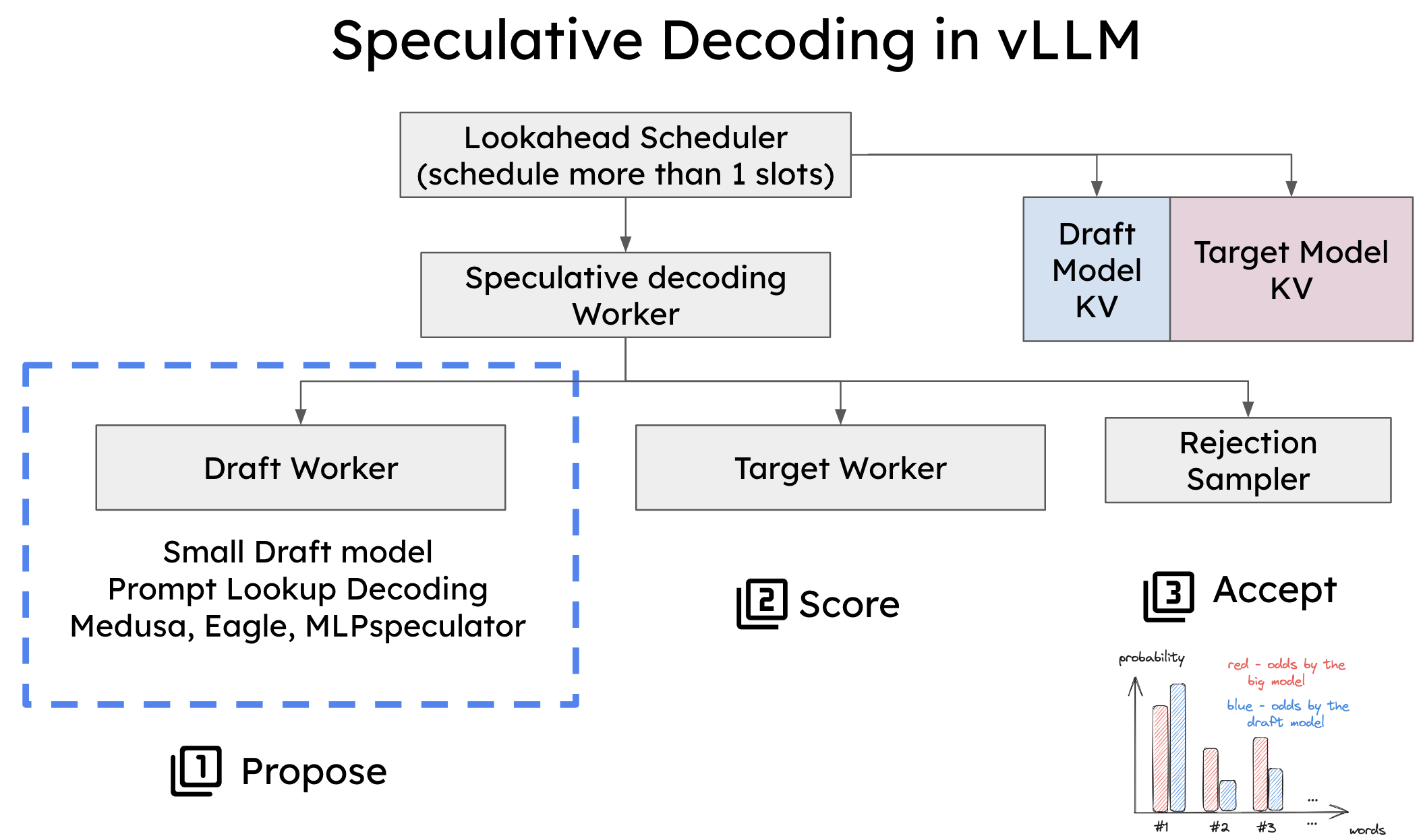
The ideal formula works best when verification exploits unused arithmetic capacity. In production, $v_\gamma$ commonly rises when:

• Baseline decode is already compute-bound. A large continuous batch may already use most tensor-core capacity, so verifying extra positions competes directly with useful work.
• $\gamma$ is too large. Long speculative spans add attention, activation, and bookkeeping work; the expected accepted length may not grow enough to justify it.
• The model is a mixture of experts. Verification may invoke more routing, dispatch, and gather overhead for the additional positions.
• Long-context or KV-heavy requests change the bottleneck. These can remain memory-bound even at substantial concurrency, but the KV-cache traffic and cache-management effects must be measured.
• The draft method is poorly integrated. Separate-model drafts may impose memory residency and scheduling costs that a lightweight draft head, prompt lookup, or $n$-gram proposer avoids.

For this reason, batch size is only a proxy. The real decision variable is whether the serving workload has headroom in compute while waiting on memory. Low-concurrency interactive chat often has that headroom; a dense-model offline batch workload may not.

A sound operational policy is dynamic:

1. Measure acceptance rate and actual accepted tokens per speculative step by workload class.
2. Measure $\tau_v(\gamma)$, draft time, and end-to-end inter-token latency across concurrency levels.
3. Select $\gamma$ from a small candidate set, rather than assuming more proposals are better.
4. Disable or reduce speculation when measured speedup is at or below $1$, or when it violates a throughput or tail-latency objective.

The most informative metric is often mean emitted tokens per target verification, because it captures both acceptance behavior and the bonus-token effect. Acceptance rate remains essential for diagnosis, but the emitted-token metric enters the speedup equation directly.

---

Key takeaways

Speculative decoding turns unused compute capacity into lower decode latency by verifying several draft positions per target-model weight pass.

• With acceptance rate $\alpha$ and $\gamma$ proposed tokens, expected emitted tokens per speculative iteration are

$$E_\gamma = \frac{1-\alpha^{\gamma+1}}{1-\alpha}$$

• Under the ideal memory-bound assumption that target verification costs one ordinary target step and one draft token costs $c$ target steps, speedup is

$$S_{\text{ideal}} = \frac{1-\alpha^{\gamma+1}} {(1-\alpha)(1+\gamma c)}$$

• In a real serving system, use measured timing:

$$S_{\text{actual}} = \frac{\tau_0 E_\gamma}{\tau_{\text{spec}}(\gamma)}$$

Speculation helps only when expected useful tokens exceed the normalized cost of drafting, verification, and overhead.

• High acceptance is valuable, but it is not sufficient by itself. Draft quality, draft cost, verifier slowdown, concurrency, model architecture, and workload shape all matter.
• The largest gains generally occur in latency-sensitive, memory-bound decode. When the GPU is already compute-saturated, speculation can reduce throughput rather than improve it.

Next, the course moves from a single decoding optimization to the serving-system level: tracing a request through gateway, admission control, routing, scheduling, model execution, and token streaming.