Inspecting Dataset Schemas and Quality with Pandas

Hello. In the previous lesson, you learned to treat a NumPy array’s shape as a contract: dimensions carry meaning, and operations must preserve that meaning. pandas builds on NumPy, but adds something crucial for real datasets: named columns, heterogeneous data types, and tools for inspecting data before modeling.

This lesson focuses on the first responsible action after receiving a CSV, spreadsheet export, or SQL query result: load it deliberately, then audit its schema and quality. The goal is not to clean anything yet. It is to produce evidence about what you actually received and how it differs from what your ML system expects.

---

A DataFrame is a labeled table, not just a matrix

A NumPy array is ideal when every value has a compatible numeric type and position defines meaning. A pandas DataFrame represents a table where each column can have a different role:

• request_id: identifier, usually text
• event_time: timestamp
• plan: categorical text
• latency_ms: numeric measurement
• converted: Boolean or binary target

The table has column labels, while the left-side index labels rows. Selecting a single column gives a pandas Series: a labeled one-dimensional object.

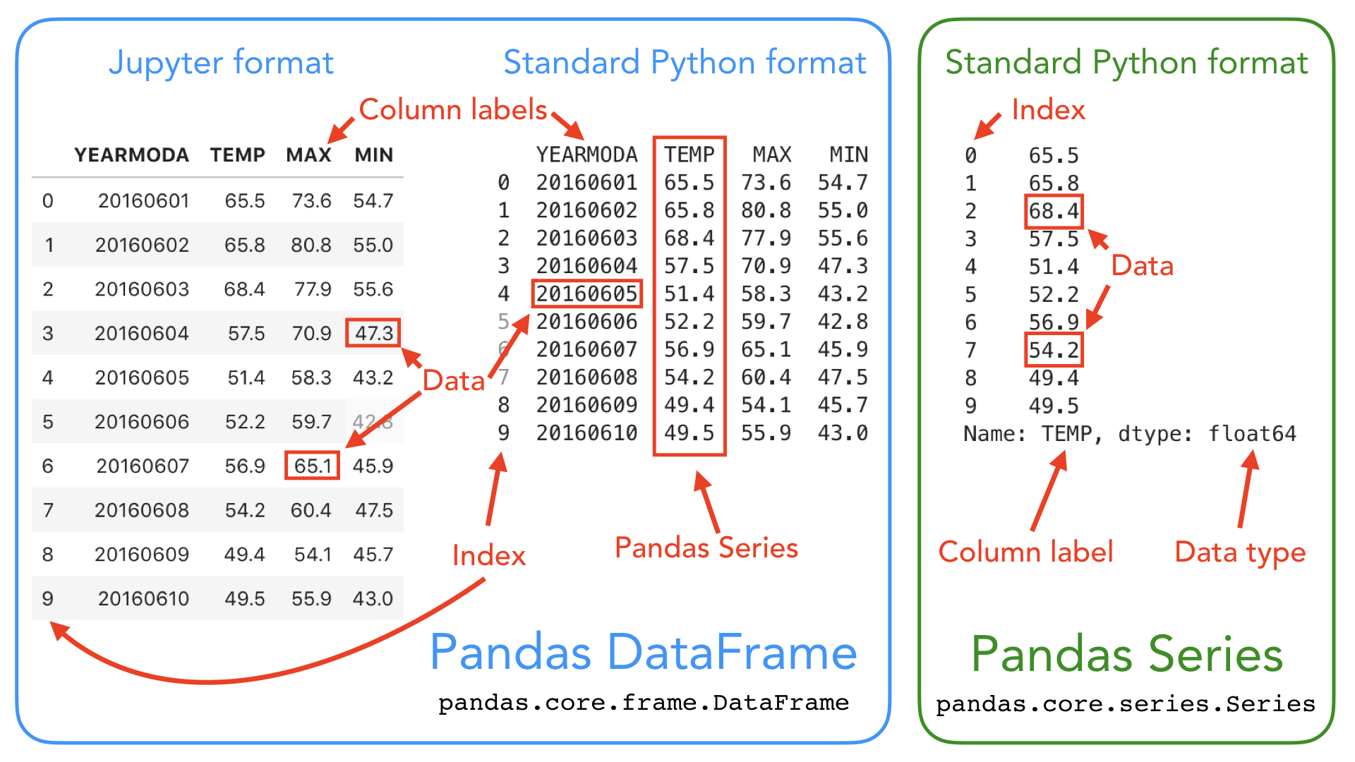
The index is useful for alignment and selection inside pandas, but it is not automatically a database primary key. When you load a normal CSV, pandas creates a RangeIndex of row positions such as 0, 1, 2, .... Keep a business identifier such as request_id as a normal column unless there is a clear reason to use it as the index.

For ML, think of a DataFrame as an intermediate representation between an external source and a model-ready feature matrix. The import boundary is where many costly errors begin:

• the wrong delimiter turns a 20-column file into one column;
• a numeric-looking identifier loses leading zeroes;
• a timestamp remains text;
• strings such as "unknown" or "N/A" are treated inconsistently;
• a stale CSV contains columns that no longer match the product schema.

Your first task is to observe these issues, record them, and avoid silently making assumptions.

---

Load data with an explicit contract

The simplest CSV import is:

import pandas as pd

df = pd.read_csv("data/raw/events.csv")

This is a good exploratory starting point for a small, familiar file. read_csv() returns a DataFrame and attempts to infer each column’s data type.

Study the loading decisions in Real Python’s guide before using them in the audit below.

Start from expectations, not from inferred types

Suppose a product team provides event data for a conversion model. Before reading deeply, write down a lightweight schema expectation:

Column	Intended meaning	Expected representation	Key check
request_id	Event identifier	string	Present and unique
user_id	User identifier	string	Leading zeroes retained
event_time	Event occurrence time	datetime	Valid timezone and format policy
plan	Subscription plan	categorical text	Known values only
latency_ms	Request latency	numeric	Non-negative
converted	Prediction target	Boolean or binary integer	Only valid labels

This is not a formal schema-validation system yet. It is an engineering hypothesis that makes inspection purposeful.

For identifiers, explicitly request strings. A value such as 001728 must remain "001728"; if parsed as an integer, it becomes 1728, destroying information.

df = pd.read_csv(
    "data/raw/events.csv",
    dtype={
        "request_id": "string",
        "user_id": "string",
        "plan": "string",
    },
)

This code deliberately leaves event_time unparsed at first. You should only ask pandas to parse dates once you know the source’s date format and semantics. If documentation and a preview confirm that the column contains valid timestamps, import it as a date:

df = pd.read_csv(
    "data/raw/events.csv",
    dtype={
        "request_id": "string",
        "user_id": "string",
        "plan": "string",
    },
    parse_dates=["event_time"],
)

If a field uses domain-specific missing markers, specify them deliberately:

df = pd.read_csv(
    "data/raw/events.csv",
    na_values={
        "country": ["unknown", "not provided"],
        "latency_ms": ["timeout", "not recorded"],
    },
)

Do not globally declare a token missing just because it looks missing. For example, "NA" might mean “not applicable,” but it could also be a valid code in a domain-specific column. The meaning belongs to the data contract, not to pandas alone.

Import failures are useful signals

A suspicious import is often visible immediately.

df = pd.read_csv("data/raw/events.csv")

print(df.shape)
print(df.columns.tolist())

If you expected 10 columns but see one, the delimiter may be wrong. A semicolon-separated source needs:

df = pd.read_csv("data/raw/events.csv", sep=";")

Another common signal is an unwanted column such as "Unnamed: 0". It frequently comes from a DataFrame index that was accidentally written into a CSV. Do not drop it automatically: first verify whether it is merely a sequential row label or a meaningful identifier.

The same inspection mindset applies to other sources:

sales = pd.read_excel("data/raw/sales.xlsx", sheet_name="transactions")

events = pd.read_sql_query(
    """
    SELECT request_id, user_id, event_time, plan, latency_ms, converted
    FROM product_events
    WHERE event_time >= '2024-01-01'
    """,
    con=engine,
)

Given your SQL experience, the read_sql_query() case should feel familiar: make the projection explicit, constrain the extraction appropriately, and inspect the resulting DataFrame rather than assuming a database column type maps perfectly to a pandas type. Once data is in a DataFrame, the following audit is the same regardless of source.

---

The initial inspection: dimensions, samples, and schema

Run a compact inspection immediately after loading:

print("Shape:", df.shape)
print("\nColumns:")
print(df.columns.tolist())

display(df.head(3))
display(df.tail(3))
display(df.sample(3, random_state=42))

df.info()

Each line answers a different question.

1. Does the table have the expected size?

df.shape

returns a tuple of:

(number_of_rows, number_of_columns)

For example, (250_000, 14) means 250,000 records and 14 columns. This is the DataFrame counterpart of NumPy’s .shape, but now each of the 14 columns may have a different type and meaning.

A surprising row count can reveal a bad SQL filter, an incomplete export, a duplicate ingestion, or a file from the wrong environment. A surprising column count often points to delimiter, header, or schema-version issues.

2. Do the beginning and end look plausible?

df.head()
df.tail()

show the first and last five rows by default. Use them to spot obvious parsing failures:

• headers appearing as the first data row;
• values shifted into the wrong columns;
• a numeric field containing an obvious text marker;
• a date field displayed as an arbitrary string;
• blank or unusual records at the end of an export.

The first rows are not necessarily representative. Inspect a reproducible random sample as well:

df.sample(5, random_state=42)

The fixed random_state makes the sample repeatable, which is useful when sharing observations with a teammate or rerunning a notebook later.

3. Does the inferred schema match the intended schema?

df.info()

is one of the most valuable pandas commands. It reports:

• the number of rows;
• each column name;
• the count of non-missing values;
• each inferred data type;
• approximate memory usage.

Watch the following focused sections of datagy’s tutorial as a quick visual walkthrough of this inspection toolkit.

A simplified .info() result might look like this:

Data columns (total 6 columns):
 #   Column      Non-Null Count   Dtype
 0   request_id  10000 non-null   string
 1   user_id     9988 non-null    string
 2   event_time  10000 non-null   object
 3   plan        9992 non-null    string
 4   latency_ms  9996 non-null    float64
 5   converted   10000 non-null   int64

Several findings deserve follow-up:

• user_id has 12 missing values despite being expected to identify an event’s user.
• event_time is object, so it was not recognized as a datetime.
• latency_ms has missing values.
• converted is numeric, but its valid set still needs checking. It might contain values other than 0 and 1.

A note about object

In older or mixed-type pandas data, object often means strings, but it is a broad fallback type. A column of currency values like "1,200.50", mixed dates, and ordinary text may all appear as object.

Therefore, do not infer meaning from the type name alone. Inspect actual values and compare them against your expected schema.

---

Audit quality without changing the data

At this stage, preserve the raw DataFrame. You are collecting evidence, not applying transformations. The next lesson will cover cleaning decisions and their consequences.

Missingness: quantify it by column

df.info() shows non-null counts, but direct counts are clearer:

missing_count = df.isna().sum()
missing_pct = (df.isna().mean() * 100).round(2)

missing_summary = pd.DataFrame({
    "missing_count": missing_count,
    "missing_pct": missing_pct,
}).sort_values("missing_count", ascending=False)

display(missing_summary)

This identifies both the amount and concentration of missingness.

Interpret missing values in context:

• A missing optional referrer may be normal.
• A missing request_id may make a record untraceable.
• A missing target label may be acceptable for future production predictions but not for supervised model training.
• Missingness concentrated in one country, device type, or date range may indicate a pipeline failure rather than ordinary absence.

For now, state the finding clearly, such as: “latency_ms is absent in 2.4% of rows; the pattern across status code and date needs investigation.” Do not yet decide whether to drop, fill, or otherwise alter it.

Duplicates: distinguish identical rows from duplicated keys

Check exact duplicate rows:

exact_duplicate_rows = df.duplicated().sum()
print(exact_duplicate_rows)

Then inspect a field expected to be unique:

duplicate_request_ids = df["request_id"].duplicated().sum()
print(duplicate_request_ids)

These checks answer different questions. Two fully identical rows can indicate repeated ingestion. Two records with the same request_id but different timestamps or status values might indicate legitimate updates, retries, or a broken identifier policy. The count is evidence; the business rule determines whether it is a defect.

Numeric values: use summaries to find implausible ranges

display(df.describe())

For numeric columns, .describe() reports count, mean, standard deviation, minimum, quartiles, and maximum. Use it to identify possible violations of the domain contract.

For example:

• a negative latency_ms is invalid;
• a percentage above 100 may be invalid, depending on its definition;
• an age of 450 is likely a data-entry error;
• a maximum order value far above the rest may be genuine, fraudulent, or incorrectly scaled.

A minimum or maximum is a signal, not a verdict. Confirm it by examining the relevant rows:

df.loc[df["latency_ms"] < 0, ["request_id", "event_time", "latency_ms"]]

The .loc selection keeps the investigation explicit: select rows matching a condition and display only the identifying and relevant fields.

Categorical values: count before assuming categories

For a low-cardinality field such as plan:

df["plan"].value_counts(dropna=False)

This reveals both distribution and suspicious variants:

free        6400
premium     2600
enterprise   850
Premium       92
premium       31
<NA>          27

Here, "premium " may contain trailing whitespace, while "Premium" differs only in capitalization. These are probably inconsistent encodings of the same category, but you should verify that assumption against product semantics before cleaning.

Use this technique carefully with high-cardinality fields such as user IDs, URLs, or free-text messages. Hundreds of thousands of unique values are expected there, and printing them all is not helpful. Instead, inspect cardinality:

df.nunique(dropna=False).sort_values()

A supposedly categorical field with almost one unique value per row may be an identifier, free text, or a column whose role has been misunderstood.

Cross-column consistency: inspect relationships that must hold

Some quality issues appear only when two columns are compared. For example, if a successful request is required to have a latency measurement:

inconsistent_rows = df[
    (df["status"] == "success") & (df["latency_ms"].isna())
]

print(inconsistent_rows.shape)

Or if converted must be binary:

df["converted"].value_counts(dropna=False)

A value such as 2, "yes", or -1 is not necessarily a parser error; it may indicate a changed source convention. Either way, it violates the expected training contract and should be recorded.

---

A repeatable first-pass audit

For an unfamiliar dataset, use this order:

1. Confirm the source and grain. What does one row represent: one user, request, transaction, session, or daily aggregate?
2. Check dimensions and column names. Compare .shape and df.columns with the expected contract.
3. Preview beginning, end, and sampled rows. Use .head(), .tail(), and reproducible .sample().
4. Inspect inferred types and completeness. Run .info(), then quantify missing values with isna().sum().
5. Inspect values by role. Use .describe() for measurements and value_counts(dropna=False) for categorical fields.
6. Test important structural assumptions. Check duplicate rows, identifier uniqueness, plausible ranges, and cross-column rules.
7. Record findings before modifying anything. A short markdown note or structured issue list is sufficient at this stage.

This process is intentionally ordinary. Its value comes from doing it every time, at the boundary where raw external data enters the ML workflow. Later, the same habits will protect training pipelines, batch inference inputs, and online inference requests.

---

Key takeaways

A pandas DataFrame combines labeled columns, a row index, and potentially mixed data types. Treat it as a structured representation of external data, not as a model-ready matrix.

Use pd.read_csv() with deliberate options when the source contract requires them: preserve identifiers as strings, define domain-specific missing markers carefully, parse dates only when justified, and investigate unexpected index-like columns or column counts.

After loading, a compact inspection using .shape, .columns, .head(), .tail(), .sample(), .info(), .describe(), isna().sum(), duplicated(), and value_counts() can reveal schema mismatches, missingness, duplicates, invalid ranges, and inconsistent categories. These methods identify problems; they do not yet solve them.

Next, you will clean missing, duplicated, and invalid DataFrame values while preserving the evidence and business rules that make each cleaning decision defensible.