Generational Garbage Collection and Performance Metrics

Welcome back. In the previous lesson, you traced a request through its thread’s stack frames and the shared heap. The key idea was reachability: an object is only shared if multiple concurrent execution paths can reach it, and it remains alive while something reachable still refers to it.

This lesson takes the next step. A Java service allocates many short-lived objects for every request: request DTOs, JSON buffers, stream pipeline objects, temporary collections, log-message data, JDBC mapping objects, and response objects. The JVM reclaims objects that are no longer reachable automatically. You will learn why it usually does that efficiently with generational garbage collection, and how to read the two operational signals that matter first: GC pause time and allocation rate.

---

From “no longer needed” to “collectible”

An object is not garbage merely because a method returned, nor because a local variable went out of scope. It is eligible for garbage collection when it is unreachable from the program’s live references, commonly called GC roots.

For the request-processing example from the previous lesson:

OrderView createOrder(CreateOrderCommand command) {
    List<OrderLine> acceptedLines = new ArrayList<>();

    for (CreateOrderLine line : command.lines()) {
        acceptedLines.add(new OrderLine(line.sku(), line.quantity()));
    }

    return new OrderView(UUID.randomUUID(), List.copyOf(acceptedLines));
}

While the method runs, its stack frame holds references to command, acceptedLines, and the objects created during processing. These references keep the objects reachable.

After the method returns:

• acceptedLines is no longer reachable if it was not returned, stored in a field, or passed to asynchronous work.
• The mutable temporary list can therefore be reclaimed in a future GC cycle.
• The returned OrderView remains reachable while the controller and JSON serializer use it.
• If a long-lived cache, singleton field, static collection, or queue retains an object, it remains reachable—even if your business logic considers it obsolete.

This is why Java can still have memory leaks: not because the JVM “forgot to free memory,” but because application code unintentionally retains references.

A collector could inspect the whole heap every time it runs and reclaim every unreachable object. But a backend process can contain millions of objects, including long-lived framework infrastructure, caches, connection-pool objects, class metadata, and active request data. Scanning all of that for every cleanup would be expensive.

Generational collection is an optimization based on an observed behavior of most Java programs:

Most objects die young.

A request creates a burst of temporary objects; most are irrelevant once the request completes. A smaller set survives longer: cached configuration, shared clients, application services, session-like state, or objects retained by queues and batches.

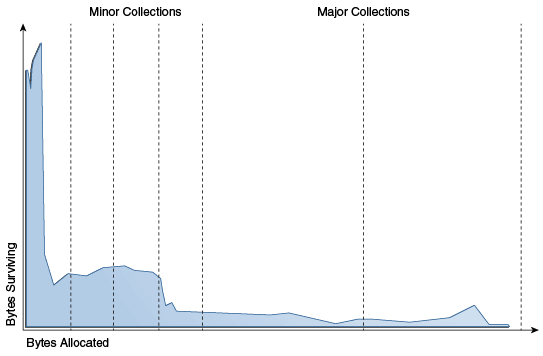
The figure is not a request timeline. Its important message is the shape: a large amount of allocated memory becomes reclaimable quickly, while a much smaller set remains alive across many allocations.

---

The generational model: young objects first

The traditional conceptual heap layout has two broad areas:

Area	Main purpose	Typical contents
Young generation	Fast reclamation of newly allocated, short-lived objects	Request-local DTOs, temporary lists, parsing buffers, short-lived stream objects
Old generation	Storage for objects that survive long enough to appear long-lived	Caches, retained domain objects, long-running batch state, framework infrastructure

The young generation is itself usually explained using three logical spaces:

1. Eden is where most new objects begin.
2. One survivor space contains objects that survived a recent young collection.
3. The other survivor space is empty and acts as the destination in the next young collection.

When Eden fills, the JVM performs a young collection, often informally called a minor GC:

• Unreachable objects in Eden are discarded.
• Reachable objects from Eden and the currently used survivor space are copied into the other survivor space.
• The previous Eden and survivor space become available for reuse.
• An object that survives several young collections may be promoted to the old generation.

Copying surviving objects is useful because it also compacts the occupied area: the survivor destination contains the live objects placed together, rather than scattered around gaps left by dead objects.

The conceptual lifecycle is:

New allocation: Eden
Young collection survival: Survivor space
Repeated survival or survivor-space pressure: Old generation
Eventually unreachable: reclaimed during an appropriate collection

The exact age at which promotion happens is a JVM decision influenced by collector behavior and survivor-space capacity. Do not treat a fixed number, such as 16 collections, as a universal rule.

For a Spring Boot service, this division maps naturally to workload behavior:

• A JSON request body parsed into DTOs is normally young and short-lived.
• A List created inside a service method is young if it does not escape.
• A static HashMap cache may begin young but will be promoted if retained.
• An accidental unbounded ConcurrentHashMap storing request information can continuously retain objects, increasing old-generation occupancy over time.

Young, major, and full collection terminology

The terminology is useful, but modern GC logs are more precise than informal labels:

• Young collection / minor collection: primarily collects young-generation objects. It is usually frequent and comparatively short because most objects there are dead.
• Old-generation collection / major collection: involves old data and generally has more work because more live objects must be considered.
• Full GC: a collector-specific term for a more comprehensive collection. It is usually an event worth investigating in a latency-sensitive backend service.

The exact implementation depends on the selected collector. On modern Java, G1 is the default collector in common JDK distributions and manages the heap as regions rather than one fixed contiguous Eden area and one fixed contiguous old area. Yet the generational mental model remains valuable: short-lived allocations are treated differently from long-lived retained data.

Also, do not use System.gc() as an application performance strategy. It is at most a request to the JVM and can produce disruptive collection work. Fix the retention or allocation behavior instead.

---

Why “more allocation” is not automatically a memory leak

Two ideas are often confused in production troubleshooting:

• Allocation rate: how many bytes the application creates per unit time.
• Live set / retained heap: how much memory remains reachable after collection.

A service can allocate several gigabytes per minute without leaking memory if most of those objects die quickly. Conversely, a service can have a modest allocation rate but still leak memory if each request retains a small object forever.

Define average allocation rate over a measurement period as:

$$\text{allocation rate}=\frac{\text{bytes allocated during the interval}}{\text{duration of the interval}}$$

For example, if a service allocates $1.2\text{ GB}$ over $60\text{ s}$, its average allocation rate is approximately:

$$\frac{1.2\text{ GB}}{60\text{ s}}=20\text{ MB/s}$$

That is a workload measurement, not an error by itself. Its significance depends on the service’s heap size, request rate, latency target, CPU budget, and GC pauses.

A practical comparison

Consider two services with the same allocation rate.

Signal	Service A: healthy temporary allocation	Service B: retention problem
Allocation rate	High	High or moderate
Heap usage after young GCs	Returns to a stable baseline	Baseline rises over time
Old-generation occupancy	Stable	Continues increasing
Full GC events	Rare or absent	Increasingly likely
Likely concern	Possibly optimize only if latency suffers	Investigate retained references and possible leak

The key distinction is the post-GC baseline. If the used heap decreases after collection and then stabilizes, the application may simply have a high temporary allocation workload. If the used heap after collection steadily climbs during equivalent traffic, some objects are surviving longer than expected.

That does not prove a leak on its own. A legitimate cache warm-up, a large import job, or a traffic mix change can increase the live set. But it tells you where to investigate.

---

Pause time: the latency signal

A GC pause is a period during which application work is stopped for a GC phase. Modern collectors can perform substantial work concurrently with the application, but they still have pause phases. For an HTTP API, a pause can add directly to request latency if it overlaps a request.

For a set of pauses $p_1,p_2,\dots ,p_n$, total pause time is:

$$P_{\text{total}}=\sum _{i=1}^n{p}_i$$

Over an observation interval $T$, the fraction of elapsed time spent paused is:

$$\text{pause fraction}=\frac{P_{\text{total}}}{T}$$

If the service experienced $900\text{ ms}$ of GC pauses in a $60\text{ s}$ load-test window:

$$\frac{0.9}{60}=0.015=1.5\%$$

That aggregate number is useful, but it can hide a user-visible outlier. A service with many $2\text{ ms}$ pauses and one $800\text{ ms}$ pause may have acceptable total pause time while still harming p99 latency.

Therefore inspect both:

• Individual pause duration, especially the maximum and upper-percentile pauses.
• Total pause time or pause fraction across a representative workload.
• Frequency of pauses, which often rises with allocation rate.
• Collection type, especially unexpected full collections.

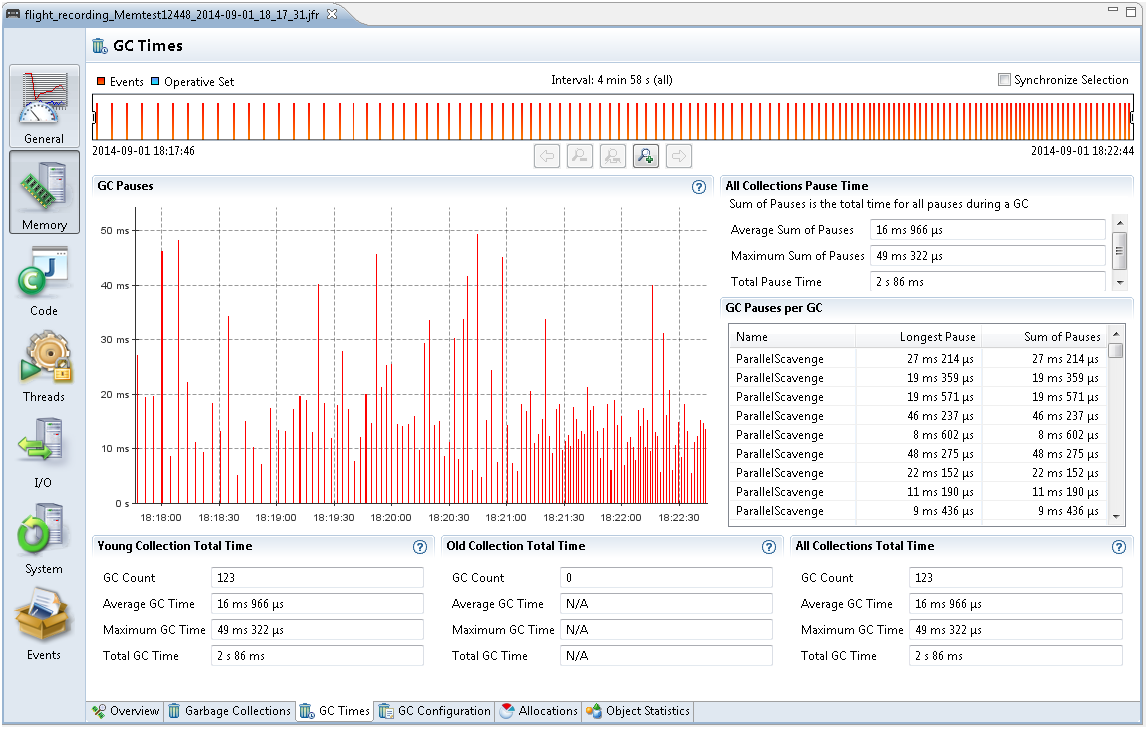
The chart above illustrates an important operational distinction:

• A tall bar indicates one potentially disruptive pause.
• A dense series of bars indicates frequent collections.
• The summary’s total pause time shows cumulative impact during the recording period.

Do not conclude that any GC pause is a production incident. The question is whether it violates a real service requirement. For example, a batch process may favor throughput and tolerate pauses that would be unacceptable for a checkout or payment endpoint.

---

Reading a basic GC log line

The JVM can emit GC logs with:

java -Xlog:gc -jar service.jar

For more diagnosis, use:

java -Xlog:gc* -jar service.jar

The first setting gives high-level collection events. The second adds details about collection phases and heap regions. Start with the simpler log; detailed logging is useful only when you have a reason to inspect a suspicious period.

A high-level G1 line commonly has this structure:

[time] GC(id) Pause Young (cause) beforeUsed->afterUsed(heapCapacity) duration

Oracle’s example includes this young collection:

Pause Young (G1 Evacuation Pause) 239M->57M(307M) ... 5.048ms

Read it in this order:

Part	Interpretation
Pause Young	A young-generation collection occurred
G1 Evacuation Pause	G1 copied live objects out of selected regions
239M	Heap memory used before the collection
57M	Heap memory used after the collection
307M	Heap capacity at that moment
5.048ms	The reported pause duration

The collection reclaimed approximately:

$$239\text{ MB}-57\text{ MB}=182\text{ MB}$$

That is generally consistent with a young collection reclaiming many temporary objects. But be careful: the remaining $57\text{ MB}$ is not automatically the survival rate of the most recent request allocations. It includes objects already live in the heap, including older objects.

A second young collection in Oracle’s example occurs after heap usage rises from roughly $57\text{ MB}$ to $238\text{ MB}$. Over the interval between those collection timestamps, that increase gives a rough indication of allocation pressure. However, GC-log heap-usage changes are only a proxy: live objects may be promoted, references may be released, and concurrent activity may occur.

For actual allocation analysis, use Java Flight Recorder allocation events and allocation-site views.

---

Measuring allocation pressure with Java Flight Recorder

A GC log tells you that collections occurred. JFR helps you connect that behavior to allocation activity in the application.

For this lesson, remember three JFR views or event families:

Signal	What it helps answer
GC Pauses	Were individual pauses too long, or was total stop time too high?
TLAB Allocations	Which classes or threads create the most small objects?
Allocation outside TLAB	Which larger allocations bypass the usual fast thread-local allocation path?
Thread Allocation Statistics	Which threads allocate the most bytes over time?

A TLAB is a Thread Local Allocation Buffer. It is a small memory area assigned to a thread so that many ordinary allocations can be performed cheaply without coordinating with every other application thread. Fast allocation does not mean free allocation: once enough objects are created, the young generation fills and GC must reclaim space.

Suppose a load test reveals that an endpoint’s allocation rate doubled after a code change. A sensible investigation order is:

1. Verify the traffic and request payloads are comparable.
2. Check whether the higher allocation rate led to more frequent young GCs or worse latency.
3. Use JFR allocation data to find the major allocating classes and threads.
4. Inspect the responsible code path for avoidable temporary objects, such as repeated JSON conversion, copying large collections, constructing unnecessary strings, or materializing a stream result several times.
5. Confirm the change improves end-to-end latency or CPU cost before keeping it.

Avoid premature micro-optimization. Replacing ordinary DTOs with obscure reusable mutable objects can create concurrency and correctness problems. In a typical microservice, first focus on allocations that are both large enough to matter and correlated with a measurable performance issue.

---

A backend diagnostic playbook

When a Java service shows slow responses, GC should be tested as a hypothesis, not assumed to be the cause. Use a representative load test, application latency metrics, GC logs, and ideally a JFR recording from the same time window.

Pattern 1: Frequent young collections, short pauses

Observed behavior

• Allocation rate is high.
• Young collections occur frequently.
• Individual pauses are short.
• The heap returns to a stable baseline after GC.

Interpretation

The service is producing many temporary objects, but the collector is reclaiming them effectively. This may be acceptable if API latency, CPU, and throughput meet requirements.

Next action

Only optimize if there is a demonstrated cost. Use JFR to find dominant allocation sites. Do not label this a memory leak just because allocation is high.

Pattern 2: A few unusually long pauses

Observed behavior

• Most requests are fast, but p99 or p99.9 latency has spikes.
• The GC pause chart has tall bars.
• A GC log may show an old or full collection around the spike.

Interpretation

A long pause may be contributing directly to tail latency. The collector choice, heap limit, CPU availability, live-set size, or application retention behavior may be relevant.

Next action

Correlate the long pause with request latency, CPU saturation, container memory limits, and old-generation occupancy. Avoid changing collector flags blindly before understanding the workload.

Pattern 3: Heap baseline climbs after each collection

Observed behavior

• Used heap after GC keeps increasing under comparable traffic.
• Old-generation occupancy trends upward.
• Full collections become more likely.
• Eventually, the process may throw OutOfMemoryError.

Interpretation

The application is retaining objects longer than expected. It could be a memory leak, an unbounded cache, an ever-growing queue, or a legitimate workload whose memory requirement exceeds the configured heap.

Next action

Capture a heap dump or use JFR/object statistics to identify what is retained and why. Increasing heap size may postpone failure, but it does not fix accidental retention.

Pattern 4: High total pause time without a single dramatic pause

Observed behavior

• No individual pause is catastrophic.
• Many pauses accumulate during the observation window.
• Throughput or latency degrades under sustained traffic.

Interpretation

Allocation pressure may be repeatedly filling the young generation, causing the application to spend too much elapsed time paused.

Next action

Investigate allocation rate and its sources. Consider heap and collector tuning only after confirming the service’s allocation behavior and container memory constraints.

---

A short hands-on runtime check

Use a small Spring Boot service or a local Java application that can receive repeated HTTP requests.

1. Start it with high-level GC logging:

   java -Xlog:gc -jar target/service.jar
   

2. Send a steady burst of comparable requests for a few minutes. A tool such as k6 is suitable because you already have experience using it.

3. In the log, note:

   • how often young collections occur,
   • the before-and-after heap values,
   • the longest reported pause,
   • whether full collections appear.

4. Repeat with a deliberately allocation-heavy endpoint if you have one, such as an endpoint that maps a large response or performs repeated serialization. Compare allocation pressure and pause frequency, not just raw request throughput.

Your goal is not to tune JVM flags today. It is to form a defensible observation such as:

“Under this request rate, the service performs frequent young collections, but pauses remain below the endpoint’s latency budget and post-GC heap usage is stable. The evidence points to temporary allocation rather than a retention issue.”

That is a far stronger production diagnosis than “GC happened, so memory is the problem.”

---

Interview revision

A concise answer to “Why does Java use generational garbage collection?” is:

Java workloads commonly follow the weak generational hypothesis: most objects become unreachable shortly after allocation. A generational collector therefore collects young objects frequently, where most memory can be reclaimed cheaply, while collecting long-lived old data less often. This reduces work compared with scanning the entire heap on every collection.

For “What is the difference between allocation rate and a memory leak?”:

Allocation rate is the number of bytes created per unit time. A high allocation rate can be healthy if those objects die young and the post-GC heap baseline stays stable. A memory leak is unintended retention: objects remain reachable, so used heap after GC and old-generation occupancy tend to rise over time.

---

Key takeaways

• An object becomes eligible for collection when it is unreachable, not simply when a method returns.
• Generational GC exploits the fact that most request-scoped objects die young.
• New objects usually begin in Eden; survivors move between survivor spaces and may later be promoted to the old generation.
• Young collections are usually frequent and relatively short. Old or full collections typically deserve more attention because they can affect tail latency.
• Allocation rate measures bytes created over time; it is not the same as retained heap usage.
• A stable post-GC heap baseline suggests temporary allocation. A steadily rising post-GC baseline suggests retention that should be investigated.
• Assess GC impact with both individual pause duration and total pause time over a representative observation window.
• GC logs answer what the JVM did; JFR helps identify which application code and threads generated allocation pressure.

Next, you will move from object lifetime to the Java Memory Model: the distinct guarantees of atomicity, visibility, and ordering when multiple threads access shared state.