Contrastive Learning for Sentence Embeddings

Hello! Welcome to the next lesson on building advanced Retrieval-Augmented Generation (RAG) systems.

In our last session, we significantly improved our RAG pipeline's precision by implementing a cross-encoder reranker. This added a crucial second stage to our retrieval process, ensuring that the documents passed to the generator were not just semantically similar but truly relevant to the query.

We've polished the second stage of retrieval, but what about the first? Our current bi-encoder is a generic, off-the-shelf model. While effective, its performance can be suboptimal on specialized or niche topics. This lesson will address that gap. Our learning goal is to apply contrastive learning to train high-quality sentence embedding models (bi-encoders). By fine-tuning our own bi-encoder, we can create a custom retriever that understands the specific nuances of our data, leading to better recall and a more powerful RAG pipeline from the very first step.

1. Why Vanilla Transformers Aren't Enough for Similarity

You might wonder why we can't just take a powerful pre-trained model like BERT and use it for sentence similarity. After all, it's a master of language understanding. However, models like BERT or RoBERTa, in their "raw" form, are not inherently optimized for generating sentence embeddings that capture semantic similarity.

A naive approach, like averaging the output token embeddings of a raw BERT model, produces surprisingly poor results. The model was pre-trained on tasks like Masked Language Modeling and Next Sentence Prediction, which don't directly teach it to create a well-structured embedding space where sentence meanings are mapped to distances.

This is why Sentence Transformers were developed. They are models like BERT that have been specifically fine-tuned on sentence-level tasks.

To understand this crucial distinction, let's start with a video that explains why BERT needs this additional training to become effective for semantic search.

As the video explains, we need to fine-tune the base model on tasks that teach it to map sentence meaning to vector space. The most powerful and widely used technique to achieve this is contrastive learning.

2. The Core Idea: Contrastive Learning

Contrastive learning is an elegant and intuitive approach to representation learning. In simple terms, it teaches a model by comparison. The goal is to organize an embedding space such that:

• Embeddings of similar items (positive pairs) are pulled closer together.
• Embeddings of dissimilar items (negative pairs) are pushed farther apart.

Imagine the embeddings as points in a high-dimensional space. Contrastive learning effectively acts like a force, attracting related points and repelling unrelated ones.

To apply this to sentences, we need three key components:

1. A way to generate positive pairs (e.g., a question and its correct answer, two paraphrases of the same sentence).
2. A way to identify negative pairs (e.g., a question and an unrelated sentence).
3. A loss function that mathematically enforces the "pull together, push apart" objective.

3. Training Architecture and Loss Function

Bi-Encoder (Siamese) Architecture

The standard architecture for this task is a bi-encoder, often referred to as a Siamese network in this context because the two encoders are identical and share the same weights.

Here's how it works during training:

1. A pair of sentences (e.g., an anchor and a positive) are fed into the network.
2. Each sentence passes through its own encoder independently.
3. This produces two sentence embeddings, u and v.
4. These embeddings are then fed into the contrastive loss function.

This is fundamentally different from the cross-encoder we studied last lesson, which processes both sentences jointly. The bi-encoder's independent processing is what makes it incredibly fast for retrieval over millions of documents.

The Contrastive Loss Function

The loss function is the engine of contrastive learning. A common and effective approach is to frame the task as a classification problem.

Imagine we have a batch of N sentence pairs (anchor_1, positive_1), (anchor_2, positive_2), ..., (anchor_N, positive_N).

1. We encode all 2N sentences to get their embeddings.
2. For a single anchor anchor_i, its corresponding positive_i is the positive example.
3. All other 2N-2 sentences in the batch are considered negative examples. This clever use of other pairs in the batch as negatives is called in-batch negatives.
4. We compute the cosine similarity between the embedding of anchor_i and all other 2N-1 embeddings.
5. We want the similarity score sim(anchor_i, positive_i) to be maximized, while the similarity scores with all negative examples are minimized.

This looks exactly like a classification problem where we want to predict the correct "class" (the positive example) out of 2N-1 possibilities. Therefore, we can use the familiar Cross-Entropy Loss to train the model. The similarity scores serve as the logits for the classification.

This specific training setup, which uses positive pairs and in-batch negatives with a classification-style loss, is often called Multiple Negatives Ranking (MNR) Loss. It is one of the most effective methods for training high-quality sentence transformers.

4. A Practical Guide to Fine-Tuning with sentence-transformers

Now, let's move from theory to practice. The sentence-transformers library, which we've used for inference, also provides powerful, high-level tools for fine-tuning models.

We'll follow a detailed video tutorial that walks through the entire process of fine-tuning a model using Multiple Negatives Ranking loss.

Step 1: Understanding the Goal and the Data

First, let's get a clear picture of MNR loss and the kind of data we need. We'll use a Natural Language Inference (NLI) dataset. An NLI dataset contains pairs of sentences (a premise and a hypothesis) labeled as entailment, neutral, or contradiction. For our purposes, a premise-hypothesis pair labeled entailment forms a perfect positive pair.

Step 2: The Training Process

With our data prepared, how does the model actually learn? The next segment of the video provides a fantastic visual explanation of the bi-encoder (Siamese) architecture in action, followed by a conceptual walkthrough of how the cosine similarity matrix is built and how the labels for the loss function are simply the indices 0, 1, 2, ... N-1 for a batch of size N.

Step 3: Implementation with the sentence-transformers Library

While the video briefly shows a raw PyTorch implementation, the sentence-transformers library abstracts all of that complexity away. The next part of the video shows how to accomplish the same task with just a few lines of code. This is the approach you will typically use in practice.

{
    "intro": "This is the most practical part of the lesson. Let's see how to implement this efficiently.",
    "resource_id": "[LINK](https://www.youtube.com/watch?v=or5ew7dqA-c)",
    "relevant_sections": [5],
    "instructions": "Watch from **22:56 to 32:29**. This section is crucial. Pay close attention to these key components:
- `InputExample`: The data structure for our sentence pairs.
- `NoDuplicatesDataLoader`: The special data loader that prevents duplicate sentences in a batch.
- `models.Transformer` and `models.Pooling`: Building the model from modules.
- `losses.MultipleNegativesRankingLoss`: The high-level implementation of the loss function we've been discussing.
- `model.fit()`: The simple, powerful training command.",
    "estimated_time": "10 minutes"
}

5. Advanced Technique: SimCSE

Contrastive learning is a vibrant area of research. One highly influential method is SimCSE (Simple Contrastive Learning of Sentence Embeddings). It introduces a clever way to perform contrastive learning even without labeled pairs.

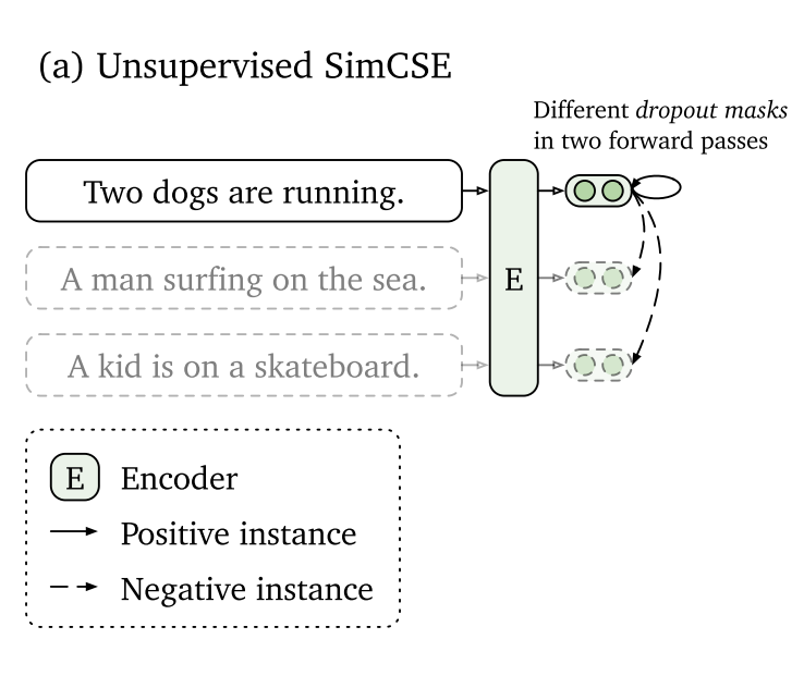
Unsupervised SimCSE: This technique creates positive pairs from a single sentence. How? By feeding the same sentence through the encoder twice. Because the model uses dropout (which randomly deactivates some neurons), it produces two slightly different embeddings. These two embeddings are treated as a positive pair. The negatives are other sentences in the batch. It's a simple but remarkably effective idea.

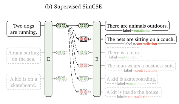
Supervised SimCSE: This method uses NLI datasets, much like the MNR example we just studied. It takes an anchor sentence (premise), its entailment sentence as a positive, and its contradiction sentence as a "hard negative" (a negative that is semantically related but opposite in meaning, making the model's job harder and the learning more robust).

These SimCSE methods are behind many top-performing sentence embedding models available today and represent a key breakthrough in the field.

Conclusion

Congratulations! You have now mastered the theory and practice of training your own high-quality bi-encoder models. This is a critical skill for building state-of-the-art retrieval systems.

Key Takeaways:

• Off-the-shelf transformer models like BERT are not directly optimized for sentence similarity. They must be fine-tuned for this task.
• Contrastive learning is the core technique for this fine-tuning. It works by pulling positive (similar) sentence pairs together and pushing negative (dissimilar) pairs apart in the embedding space.
• The bi-encoder (Siamese) architecture is used for training, processing sentences independently to produce embeddings that are then compared by a loss function.
• Multiple Negatives Ranking (MNR) Loss is an efficient and powerful contrastive loss function that uses a classification-style objective (Cross-Entropy Loss) with in-batch negatives.
• The sentence-transformers library provides high-level APIs like MultipleNegativesRankingLoss and model.fit() that make fine-tuning these models incredibly accessible.

Preview of the Next Lesson:

We have now explored the full, advanced RAG pipeline: a fine-tuned retriever for high recall and a cross-encoder for high-precision reranking. But how do we know if our improvements are actually working? Building great systems requires measuring them. In our next lesson, we will focus on evaluating RAG systems, covering both retrieval metrics (e.g., MRR, NDCG) and generation metrics to get a complete picture of our pipeline's performance.